Rigid Body Kinematics in 3D Space
Moses C. Nah
2023-03-06
Introduction
Here, we discuss about rigid body kinematics in 3D space. Before going through the post, I highly recommend to read through this post and its following posts in great detail. First and foremost, we discuss about rotational motion in 3D space.
Euler’s Rotation Theorem
Euler’s rotation theorem establishes the foundation of rotational motion in 3D space. The theorem states that:
In three-dimensional space, any displacement of a rigid body such that a point on the rigid body remains fixed, is equivalent to a single rotation about some axis that runs through the fixed point.
The proof of this theorem is shown in this post using the properties of rotation matrices.
Based on Euler’s rotation theorem, one can define the angular velocity of the rigid object. Let the arbitrary rotation of a rigid object be described as a unit axis of rotation \(\hat{\boldsymbol{\omega}}\in\mathbb{R}^{3}\) and its amount of rotation \(\theta\in\mathbb{R}\).
If we consider an infinitesimal rotation \(d\theta\) about axis \(\hat{\boldsymbol{\omega}}\), the rate of change provides us the angular velocity \(\boldsymbol{\omega}\). \[ \boldsymbol{\omega} := \frac{d\theta}{dt} \hat{\boldsymbol{\omega}} = \dot{\theta} \hat{\boldsymbol{\omega}}, ~~~~~~~~~~ \dot{\theta} = \lim_{\Delta t\rightarrow 0}\frac{\Delta \theta}{\Delta t} \] Note that angular velocity does not need a reference point. Hence, as with force vector subscripts are not required for angular velocity.1 Taking account for this fact becomes useful when we discuss about superposition principle of angular velocities.
Kinematics of an Arbitrary Point of a Rigid Object
Based on the definition of angular velocity, we can calculate the velocity and acceleration of an arbitrary point attached to a rigid object. Consider point \(A\) and \(B\) attached to the rigid object (Figure 1). The simple kinematic relation is \(\mathbf{r}_B = \mathbf{r}_A + \mathbf{r}'\). We consider two frames: a fixed, inertial frame \(\{S\}\) and a body-fixed frame \(\{B\}\) attached to the body. Let the position of point \(B\) from point \(A\) with respect to frame \(\{S\}\) and \(\{B\}\), \({}^{s}\mathbf{r}', {}^{b}\mathbf{r}'\) be: \[ {}^{s}\mathbf{r}' = {}^{s}x'\mathrm{\hat{e}_X}+{}^{s}y'\mathrm{\hat{e}_Y}+{}^{s}z'\mathrm{\hat{e}_Z} ~~~~~~~~~~~~ {}^{b}\mathbf{r}' = {}^{b}x'\mathrm{\hat{e}_1}+{}^{b}y'\mathrm{\hat{e}_2}+{}^{b}z'\mathrm{\hat{e}_3} \] Let the velocity of point \(A\) with respect to frame \(\{S\}\) be \({}^{s}\mathbf{v}_A\). The velocity of point \(B\) with respect to frame \(\{S\}\) is: \[ {}^{s}\mathbf{v}_B = {}^{s}\mathbf{v}_A + \frac{d}{dt}{}^{s}\mathbf{r}' \] Rather than taking the time derivative of \({}^{s}\mathbf{r}'\), we exploit the fact that the object is a rigid object, and thus the components of \({}^{s}\mathbf{r}'\) is fixed with respect to time. However, as shown in this section of the post, one might consider the time derivatives of bases \(\mathrm{\hat{e}_1}, \mathrm{\hat{e}_2}, \mathrm{\hat{e}_3}\). This derivation can be succinctly expressed using rotation matrix \({}^{s}\mathbf{R}_b\):2
\[ {}^{s}\mathbf{v}_B = {}^{s}\mathbf{v}_A + \frac{d}{dt}{}^{s}\mathbf{r}' = {}^{s}\mathbf{v}_A + \frac{d}{dt}\big({}^{s}\mathbf{R}_b{}^{b}\mathbf{r}'\big) = {}^{s}\mathbf{v}_A +{}^{s}\mathbf{\dot{R}}_b{}^{b}\mathbf{r}' = {}^{s}\mathbf{v}_A + \underbrace{ {}^{s}\mathbf{\dot{R}}_b {}^{b}\mathbf{R}_s }_{=[{}^{s}\boldsymbol{\omega}]} ~\underbrace{{}^{s}\mathbf{R}_b{}^{b} \mathbf{r}'}_{={}^{s}\mathbf{r}'} = {}^{s}\mathbf{v}_A + {}^{s}\boldsymbol{\omega} \times {}^{s}\mathbf{r}' \] Hence, with respect to the inertial reference frame \(\{S\}\), we have the following kinematic relation: \[ {}^{s}\mathbf{v}_B = {}^{s}\mathbf{v}_A + {}^{s}\boldsymbol{\omega} \times {}^{s}\mathbf{r}' \]
The derivation of the acceleration of point \(B\) is also straightforward. Let the acceleration of point \(A\) with respect to frame \(\{S\}\) be \({}^{s}\mathbf{a}_A\). The acceleration of point \(B\) with respect to frame \(\{S\}\) is: \[ \begin{align} {}^{s}\mathbf{a}_B &= {}^{s}\mathbf{a}_A + \Big(\frac{d}{dt}{}^{s}\boldsymbol{\omega} \Big) \times {}^{s}\mathbf{r}' + {}^{s}\boldsymbol{\omega} \times \Big( \frac{d}{dt} {}^{s}\mathbf{r}' \Big) = {}^{s}\mathbf{a}_A + \Big(\frac{d}{dt}{}^{s}\boldsymbol{\omega} \Big) \times {}^{s}\mathbf{r}' + {}^{s}\boldsymbol{\omega} \times \big( {}^{s}\boldsymbol{\omega} \times {}^{s}\mathbf{r}' \big) \end{align} \]
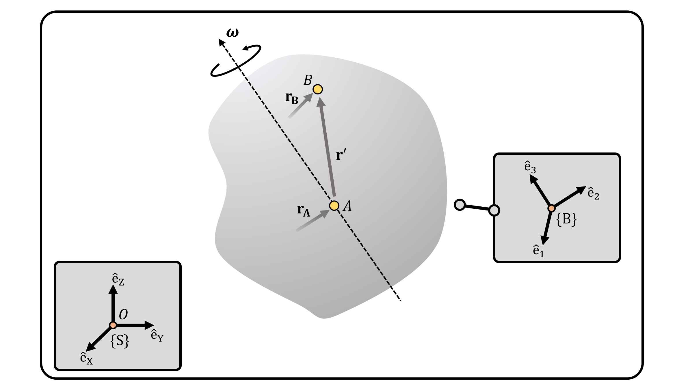
(Figure 1)
Remarks
Some important remarks are made. Equality symbol should be used with care.
References
Hence, it is simply wrong to say angular velocity of the rigid object “about point A.”↩︎
Note that to multiply \({}^{s}\mathbf{R}_b\in\mathbb{R}^{3\times 3}\) with \({}^{b}\mathbf{r}'\), we simply stack the components of \({}^{b}\mathbf{r}'\) as a \(\mathbb{R}^{3}\) array. In detail: \[ {}^{s}\mathbf{r}' = \begin{bmatrix} {}^{s}x' \\ {}^{s}y' \\ {}^{s}z' \end{bmatrix}, ~~~~ {}^{b}\mathbf{r}' = \begin{bmatrix} {}^{b}x' \\ {}^{b}y' \\ {}^{b}z' \end{bmatrix} \] Nevertheless, care if required when adding up \(\mathbb{R}^{3}\) arrays. To add or subtract \(\mathbb{R}^{3}\) arrays one may keep in mind that the components are with respect to the same bases.↩︎