Moment of Inertia

Definition of Moment of Inertia

Consider a rigid object consisting of \(N\) particles. Let the object be fixed at point \(A\), i.e., the object can freely rotate about point \(A\) (Figure 1). Let the angular velocity of the rigid object be \(\boldsymbol{\omega}\in\mathbb{R}^3\). The velocity of the \(i\)-th particle with mass \(m_i\), located at \(\mathbf{r}_i\) is: \[ \mathbf{v}_i = \boldsymbol{\omega} \times \mathbf{r}_i, \;\;\;\; \mathbf{v}_i = \begin{bmatrix} 0 & -\omega_z & \omega_y \\ \omega_z & 0 & -\omega_x \\ -\omega_y & \omega_x & 0 \end{bmatrix} \begin{bmatrix} x_i \\ y_i \\ z_i \end{bmatrix} := [\boldsymbol{\omega}]\mathbf{r}_i \] where the second equation uses the matrix representation of the cross product of vectors.¹

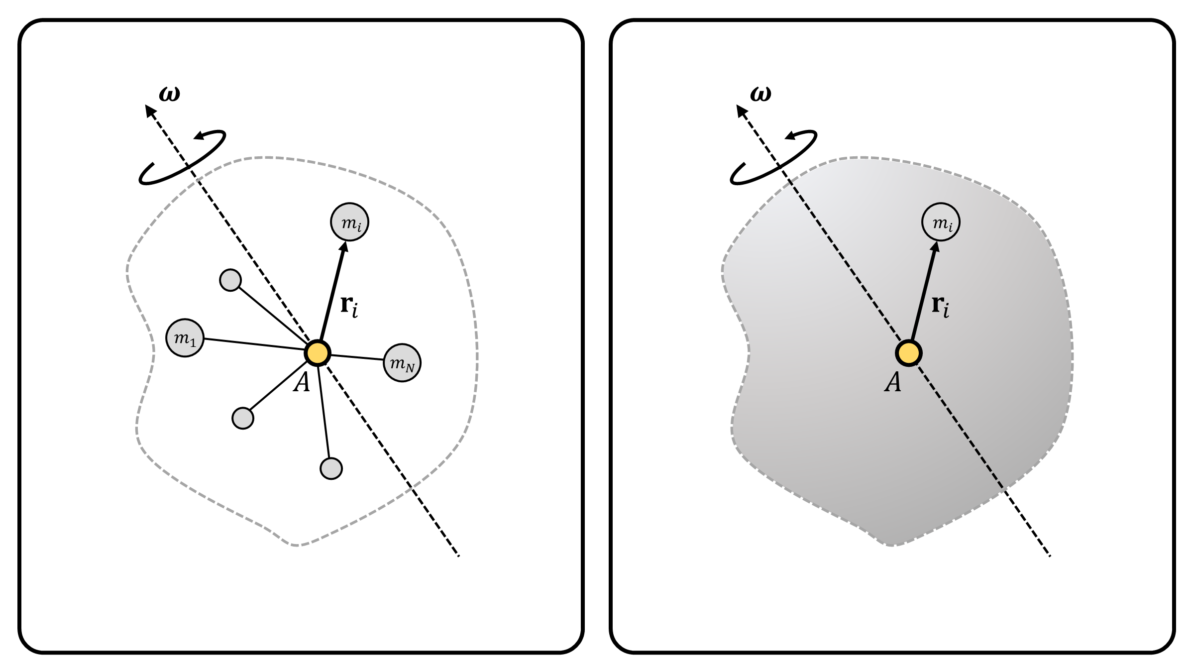
(Figure 1) (Left) A rigid object consisting of \(N\) mass particles, fixed at point \(A\). The angular velocity of the rigid object is \(\boldsymbol{\omega}\). (Right) A simplified depiction of rigid object on left.

Based on the definition of angular momentum, the angular momentum of the \(i\)-th mass, \(m_i\) about point \(A\) is: \[ \mathbf{H}_{A,i} := \mathbf{r}_i \times \mathbf{p}_i = \mathbf{r}_i \times m_i\mathbf{v}_i \; = \mathbf{r}_i \times (\mathbf{\boldsymbol{\omega} \times r_i }) \; m_i \] Using the matrix representation of cross product, we further simplify integrate the equations:^{2 3} \[ \begin{align*} \mathbf{H}_{A,i} &= \mathbf{r}_i \times (\mathbf{\boldsymbol{\omega} \times r_i })~m_i = [\mathbf{r}_i][\boldsymbol{\omega}]\mathbf{r}_i~ m_i = -[\mathbf{r}_i][\mathbf{r}_i]\boldsymbol{\omega}~m_i = -m_i[\mathbf{r}_i]^2\boldsymbol{\omega} \\ \mathbf{H}_A &= \sum_{i=1}^{N}\mathbf{H}_{A,i}= \Big( \sum_{i=1}^{N} -m_i[\mathbf{r}_i]^2 \big)\boldsymbol{\omega} := \mathbf{I}_A\boldsymbol{\omega} \end{align*} \]

We call the \(\mathbf{I}_A\in\mathbb{R}^{3\times 3}\) matrix the moment of inertia of the rigid object about point \(A\): \[ \mathbf{H}_A = \mathbf{I}_A\boldsymbol{\omega} \tag{1} \] To the best of the author’s knowledge, this is the most concise definition of moment of inertia. Note that Equation 1 is reminisent of the linear momentum principle, \(\mathbf{p}=m\mathbf{v}\), where \(\mathbf{I}_A\) and \(\boldsymbol{\omega}\) correspond to mass \(m\) and linear velocity \(\mathbf{v}\), respectively.

The moment of inertia can be reformulated: \[ \mathbf{I}_A = \sum_{i=1}^{N} m_i\big(-[\mathbf{r}_i]^2\big) = \sum_{i=1}^{N} m_i \big( ||\mathbf{r}_i||^2\mathbf{I}_3-\mathbf{r_ir_i^T} \big) = \sum_{i=1}^{N} m_i\Big( \text{tr}(\mathbf{r_ir_i^T})\mathbf{I}_3 -\mathbf{r_ir_i^T} \Big) \] Each component of the inertia matrix about point \(A\) is: \[ \mathbf{I}_A = \begin{bmatrix} \sum_{i=1}^{N} m_i(y_i^2+z_i^2) & -\sum_{i=1}^{N} m_i x_iy_i & -\sum_{i=1}^{N} m_ix_iz_i \\ -\sum_{i=1}^{N} m_ix_iy_i & \sum_{i=1}^{N} m_i(x_i^2+z_i^2) & -\sum_{i=1}^{N} m_iy_iz_i \\ -\sum_{i=1}^{N} m_ix_iz_i & -\sum_{i=1}^{N} m_iy_iz_i & \sum_{i=1}^{N} m_i(x_i^2+y_i^2) \end{bmatrix}:= \begin{bmatrix} \phantom{-}I_{A,xx} & -I_{A,xy} & -I_{A,xz} \\ -I_{A,xy} & \phantom{-}I_{A,yy} & -I_{A,yz} \\ -I_{A,xz} & -I_{A,yz} & \phantom{-}I_{A,zz} \end{bmatrix} \tag{2} \] where \(\mathbf{r}_{i}=[x_i, y_i, x_i]\) is the position of the \(i\)-th particle measured from point \(A\). Note that by definition, the moment of inertia of the rigid object is a symmetric matrix.⁴ Moreover, it is immediate that for a rigid object with discrete distribution of masses, summation changes to an integration with respect to the mass density function. Finally, it is clear that to define the three components of \(\mathbf{r}_i\), one should define a reference frame fixed at point \(A\).

Principal Axes and Principal Moments of Inertia

Since the inertia matrix is by definition a symmetric matrix, based on spectral theorem, one can always find three mutually orthonormal eigenvectors⁵ of the inertia matrix, and the corresponding eigenvalues with real values. The eigenvectors of the inertia matrix are called the principal axes of inertia, and the corresponding eigenvalues are called the principal moments of inertia.⁶

In detail, let \(\mathbf{v}_1\),\(\mathbf{v}_2\),\(\mathbf{v}_3\) be the principal axes of inertia (i.e., three mutually orthonormal eigenvectors) of inertia matrix \(\mathbf{I}_A\), and let \(I_1\), \(I_2\), \(I_3\) be the corresponding principal moments of inertia (i.e., the corresponding eigenvalues of the eigenvectors), respectively. Then: \[ \mathbf{I}_A\mathbf{v}_1 = I_1\mathbf{v}_1 ~~~~~~~~~ \mathbf{I}_A\mathbf{v}_2 = I_2\mathbf{v}_2 ~~~~~~~~~ \mathbf{I}_A\mathbf{v}_3 = I_3\mathbf{v}_3 \tag{3} \] It is clear that rotation in 3D space is difficult that the rotation in 2D space, since the angular momentum \(\mathbf{H}_A\) is not always parallel to the angular velocity \(\boldsymbol{\omega}\). However, if the angular velocity of the rigid object is along one of the principal axes of inertia, the angular momentum is parallel to the angular velocity.

Using rotation matrices, or an element of a Special Orthogonal Group SO(3) \(\mathbf{R}\in SO(3)\), Equation 3 can be expressed as: \[ \mathbf{I}_A \underbrace{ \begin{bmatrix} \vert & \vert & \vert \\ \mathbf{v}_1 & \mathbf{v}_2 & \mathbf{v_3} \\ \vert & \vert & \vert \\ \end{bmatrix} }_{:=\mathbf{R}\in SO(3)} = \begin{bmatrix} \vert & \vert & \vert \\ \mathbf{v}_1 & \mathbf{v}_2 & \mathbf{v_3} \\ \vert & \vert & \vert \\ \end{bmatrix} \underbrace{ \begin{bmatrix} I_1 & & \\ & I_2 & \\ & & I_3 \\ \end{bmatrix}}_{:=\mathbf{I}_A'} ~~~~~~~~~~~~ \mathbf{I}_A = \mathbf{R}\mathbf{I}_A'\mathbf{R^{T}} \tag{3} \]

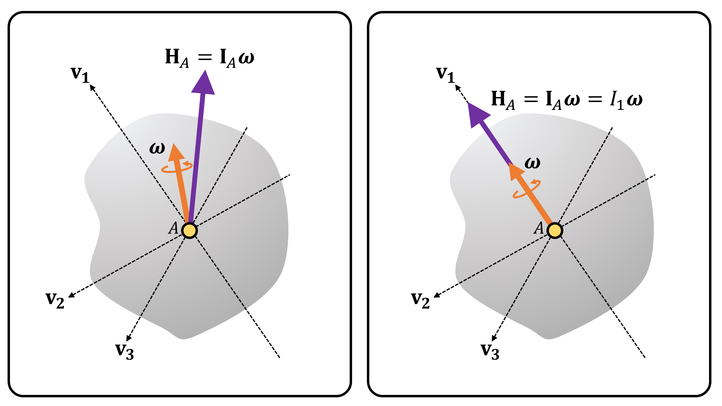
(Figure 2) A rigid object with arbitrary shape, fixed at point \(A\). Dotted lines \(\mathbf{v}_1\), \(\mathbf{v}_2\), \(\mathbf{v}_3\) depict the principal axes of inertia of the rigid object. (Left) If the angular velocity is not aligned with one of the principal axes of inertia, the angular momentum of the object about point \(A\) is not aligned with the angular velocity. (Right) If the angular velocity is aligned with one of the principal axes of inertia, the angular momentum of the object about point \(A\) is aligned with the angular velocity.

Triangular Inequalities of the Inertia Matrix

Based on the definition of inertia matrix \(\mathbf{I}_A\), it is clear that the inertia matrix should be a positive definite matrix: \[ \mathbf{I}_A := \sum_{i=1}^{N} m_i \big(-[\mathbf{r}_i]^2\big) = m_i \sum_{i=1}^{N} [\mathbf{r}_i]^{\mathbf{T}}[\mathbf{r}_i] ~~~~~~~~~~ \forall \mathbf{v}\in\mathbb{R}^3\setminus\{\mathbf{0}\}: \mathbf{v^T I_A v} =m_i \sum_{i=1}^{N} \big([\mathbf{r}_i]\mathbf{v}\big)^{\mathbf{T}}\big([\mathbf{r}_i]\mathbf{v}\big) > 0 \]

However, one should be aware that there is another condition which the inertia matrix should satisfy [1]. As shown in Equation 3, there always exists a special orthogonal matrix \(\mathbf{R}\in SO(3)\), which can decompose a inertia matrix as \(\mathbf{I}_A=\mathbf{R}\mathbf{I}_A'\mathbf{R^T}\), where \(\mathbf{I}_A'\) is a diagonal matrix which takes the principal moments of inertia \(I_1, I_2, I_3\) as the diagonal element. In other words, we find a new reference frame where the bases are along the principal axes of inertia. This means that: \[ \mathbf{I}_A' = \begin{bmatrix} I_1 & 0 & 0 \\ 0 & I_2 & 0 \\ 0 & 0 & I_3 \end{bmatrix} \] where each element is: \[ I_1 = \sum_{i=1}^{N}m_i(y_i'^2+z_i'^2) ~~~~~~~~~~~ I_2 = \sum_{i=1}^{N}m_i(x_i'^2+z_i'^2) ~~~~~~~~~~~ I_3 = \sum_{i=1}^{N}m_i(x_i'^2+y_i'^2) \] In these equations, \(x_i', y_i', z_i'\) are the components along the principal axes of inertia. We define the corresponding central second moments of mass [1], \(J_1, J_2, J_3\), defined by: \[ J_1 = \sum_{i=1}^{N}m_ix_i'^2 ~~~~~~~~~~~ J_2 = \sum_{i=1}^{N}m_iy_i'^2 ~~~~~~~~~~~ J_3 = \sum_{i=1}^{N}m_iz_i'^2 \tag{4} \]

Based on Equation 4, the principal moments of inertia can be reformulated as: \[ I_1 = J_2 + J_3 ~~~~~~~~~~~ I_2 = J_1 + J_3 ~~~~~~~~~~~ I_3 = J_1 + J_2 \] Since \(J_1, J_2, J_3\) are positive values, it is clear that \(I_1, I_2, I_3\) satisfies the triangular inequality: \[ I_1 + I_2 > I_3 ~~~~~~ I_2 + I_3 > I_1 ~~~~~~ I_3 + I_1 > I_2 \]

Rotational Kinetic Energy of a Rigid Object

The kinetic energy of the rigid object, which is fixed at some point \(A\), can be expressed in terms of the moment of inertia about point \(A\).

Consider the system shown in Figure 1. The total kinetic energy due to rotation \(T_r\) is the summation of the kinetic energies of the \(N\) particles: \[ T_r = \sum_{i=1}^{N}\frac{1}{2}m_i \mathbf{v}_i\cdot \mathbf{v}_i = \sum_{i=1}^{N}\frac{1}{2}m_i \mathbf{v}_i^\text{T} \mathbf{v}_i \]

Since \(\mathbf{v}_i=\boldsymbol{\omega} \times\mathbf{r}_i=-[\mathbf{r}_i]\boldsymbol{\omega}\), and \([\mathbf{r}_i]^{\text{T}}=-[\mathbf{r}_i]\): \[ T_r = \sum_{i=1}^{N}\frac{1}{2}m_i \mathbf{v}_i^\text{T} \mathbf{v}_i = \sum_{i=1}^{N}\frac{1}{2}m_i \boldsymbol{\omega}^\text{T} [\mathbf{r}_i]^{\text{T}}[\mathbf{r}_i]\boldsymbol{\omega} = \frac{1}{2}\boldsymbol{\omega}^\text{T} \underbrace{\Big( -\sum_{i=1}^{N} m_i[\mathbf{r}_i]^2 \Big)}_{:=\mathbf{I}_A}\boldsymbol{\omega} = \frac{1}{2}\boldsymbol{\omega}^\text{T}\mathbf{I}_A\boldsymbol{\omega} \]

We call \(T_r\) the rotational kinetic energy of a rotating rigid body.

Parallel Axis Theorem

Consider the rigid object in Figure 1. We now choose point \(A\) to be the center of mass of the object, which we refer to as point \(C\). Given a reference frame at point \(C\), let the inertia matrix of the rigid object about point \(C\) be \(\mathbf{I}_C\).

Parallel axis theorem, also known as Huygens—Steiner theorem derives the relation between the moment of inertia about the center of mass, and the moment of inertia about any point. But the moment of inertia is defined about the same reference frame, i.e., as if we parallel shifted the reference frame from the center of mass to the point in interest.

Consider we define a new point \(B\) as shown in Figure 3. A simple kinematic relation show that \(\mathbf{r}_i = \mathbf{r}_i' + \mathbf{r}\), where \(\mathbf{r}_i'\) is the position of the \(i\)-th particle measured from point \(B\), and \(\mathbf{r}\) is the location of point \(B\) measured from point \(C\). Note that the frame attached at point \(C\) and \(B\) are identical, since it is parallel shifted.

By definition of the moment of inertia about \(B\), and using the kinematic relation: \[ \begin{align*} \mathbf{I}_B &= \sum_{i=1}^{N} m_i\big(-[\mathbf{r}_i']^2\big) = \sum_{i=1}^{N} m_i\big(-[\mathbf{r}_i - \mathbf{r}]^2\big) = \sum_{i=1}^{N} m_i\big(-\{[\mathbf{r}_i] - [ \mathbf{r}]\}^2\big) \\ &= \underbrace{\sum_{i=1}^{N} m_i\big(-[\mathbf{r}_i]^2\big)}_{:=\mathbf{I}_C} + \sum_{i=1}^{N} m_i\big(-[\mathbf{r}]^2\big) + 2\Big(\sum_{i=1}^{N}m_i[\mathbf{r}_i]\Big)[\mathbf{r}] \end{align*} \] By definition of the center of mass, i.e., based on Equation 2 in this post:⁷ \[ \sum_{i=1}^{N}m_i\mathbf{r}_i = \mathbf{0} ~~~~~~ \text{or} ~~~~~~ \sum_{i=1}^{N}m_i[\mathbf{r}_i] = \mathbf{0} \]

We derived the equation for parallel axis theorem: \[ \mathbf{I}_B = \mathbf{I}_C + \sum_{i=1}^{N} m_i\big(-[\mathbf{r}]^2\big) = \mathbf{I}_C + M\big(-[\mathbf{r}]^2\big) \tag{5} \] The mistake people often make is using the parallel axis theorem for any arbitrary two points. I may warn you that the parallel axis theorem should be always used with respect to the center of mass of the rigid object. For the right-hand side of Equation 5, the point is respect to \(C\) (center of mass).

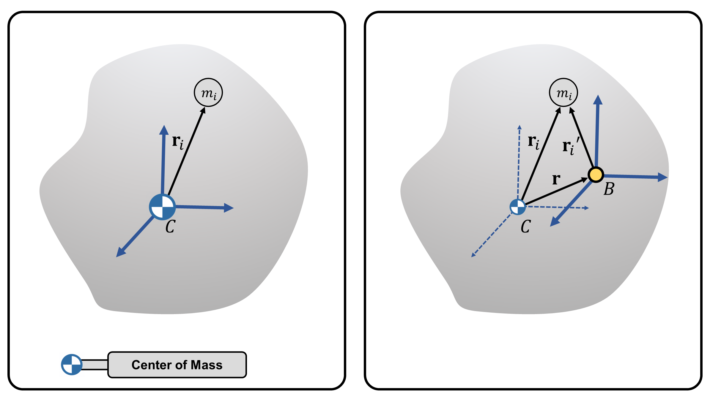
(Figure 3) (Left) A rigid object with center of mass at point \(C\). (Right) Point \(B\) with the same frame attached at point \(C\).

A Simple Example

From the center of mass of the object, let \(B\) be the point that is located at \(\mathbf{r}=[0,0,d]\). Based on parallel axis theorem, the moment of inertia about point \(B\) is: \[ \mathbf{I}_B = \mathbf{I}_C + M \Bigg(- \begin{bmatrix} 0 & -d & 0 \\ d & 0 & 0 \\ 0 & 0 & 0 \end{bmatrix} \begin{bmatrix} 0 & -d & 0 \\ d & 0 & 0 \\ 0 & 0 & 0 \end{bmatrix}\Bigg) = \mathbf{I}_C + M \begin{bmatrix} d^2 & 0 & 0 \\ 0 & d^2 & 0 \\ 0 & 0 & 0 \end{bmatrix} \]

[1]

S. Traversaro, S. Brossette, A. Escande, and F. Nori, “Identification of fully physical consistent inertial parameters using optimization on manifolds,” in 2016 IEEE/RSJ international conference on intelligent robots and systems (IROS), 2016, pp. 5446–5451.

---

1. You might find this footnote useful↩︎

2. We use the following trick: \[ \mathbf{a} \times \mathbf{b} = - \mathbf{b} \times \mathbf{a} \;\;\;\;\;\;\;\;\;\; [\mathbf{a}] \mathbf{b} = - [\mathbf{b}] \mathbf{a} \]↩︎

3. We can also use the BAC-CAB formula: \[ \mathbf{r}_i \times (\mathbf{\boldsymbol{\omega} \times r_i }) = \boldsymbol{\omega}(\mathbf{r}_i\cdot \mathbf{r}_i) - \mathbf{r}_i(\boldsymbol{\omega}\times \mathbf{r}_i) = \Big(||\mathbf{r}_i||^2\mathbf{I}_3-\mathbf{r_ir_i^T}\Big)\boldsymbol{\omega} \]↩︎

4. And in fact, it is a symmetric positive-definite matrix.↩︎

5. Note that if an eigenvector exists, then we can freely scale the eigenvector as a unit vector. ↩︎

6. Strictly speaking, the inertia matrix is a metric, a (0,2)-tensor. Hence it should rather be called a signature rather than an eigenvalue. However, in this series of posts we intentionally do not discuss about this in great detail.↩︎

7. Again, even though both equations use the same zeros, the equation used on the left-hand side is a zero vector, and the equation used on the right-hand side is a zero matrix.↩︎