Euler’s Laws of Motion and the Center of Mass
Moses C. Nah
2023-03-06
Prelude
Read Euler, read Euler, he is the master of us all.
So far, we have been focusing on studying the dynamics of a single particle, where the size of the particle itself is neglected. Hence, a motion of a particle is idealized as a motion of a point in space. Here, we focus on rigid object which is an idealization of a body that does not deform or change shape. While the analysis of the motion of rigid object is also discussed in Analytical mechanics, here we start the discussion by introducing Euler’s Laws of motion.
The rigid object can either be a continuous or discrete distribution of masses. For continuous distribution of masses, a mass density function is defined at each point of the rigid object and integration is used to calculate the total mass. For discrete distribution of masses, the system can be treated as a system of particles with different masses. In these series of posts, we focus on rigid object with discrete distribution of masses, although the principle can be immediately generalized to the case of continuous distribution of masses.
Euler’s Laws of Motion
Some textbook derives Euler’s Laws of motion from Newton’s Laws of motion using Newton’s Third Law of action-reaction, especially the strong law of action and reaction [1]. Nevertheless, as with Newton’s Laws of motion, Euler’s Laws of motions can be regarded as Axioms [2].1 Euler’s laws of motions for rigid object are as follows:
First Law (Linear Momentum Principle for Rigid Object) — In an inertial frame of reference, the rate of change of the total linear momentum of a rigid body \(\mathbf{P}\) is equal to the resultant of all the external forces acting on the rigid body: \[ \sum \mathbf{F}_{ext} = \frac{d\mathbf{P}}{dt} \]
Second Law (Angular Momentum Principle for Rigid Object) — In an inertial frame of reference, the rate of change of the total angular momentum \(\mathbf{H}_A\) about a fixed point \(A\) is equal to the sum of the external moments of force (or torques) acting on that body \(\boldsymbol{\tau}_{ext,A}\) about that point: \[ \sum \boldsymbol{\tau}_{ext,A} = \frac{d\mathbf{H}_A}{dt} \]
In this post, we mainly focus on Euler’s First Law of motion. The thorough discussion about Euler’s Second law of motion is deferred to the subsequent post. To achieve thorough understanding of Euler’s First Laws of motion, we first introduce the Center of Mass (COM) of the rigid object.
The Center of Mass (COM)
Consider a rigid object which consists of a set of \(N\) particles (Figure 1). Let the total mass of the object be \(\mathbf{M}:=\sum m_i\). The center of mass of this object, \(\mathbf{R}\) is an abstract mathematical point, defined by:2 \[ \mathbf{R} := \frac{\sum_{i=1}^{N}m_i\mathbf{r_i}}{\sum_{i=1}^{N}m_i} = \frac{\sum_{i=1}^{N}m_i\mathbf{r_i}}{M} \tag{1} \] The center of mass is a weighted average of the positions of all parts of the system, where each weight corresponds to the mass of each part.
Note that we can reformulate Equation 1 as: \[ \sum_{i=1}^{N}m_i\mathbf{R} = \sum_{i=1}^{N}m_i\mathbf{r_i} ~~~~~~~~~~~~~~~~ \sum_{i=1}^{N}m_i(\mathbf{R}-\mathbf{r}_i) = 0 \tag{2} \] This property is useful when we discuss about Euler’s Second Law of motion.
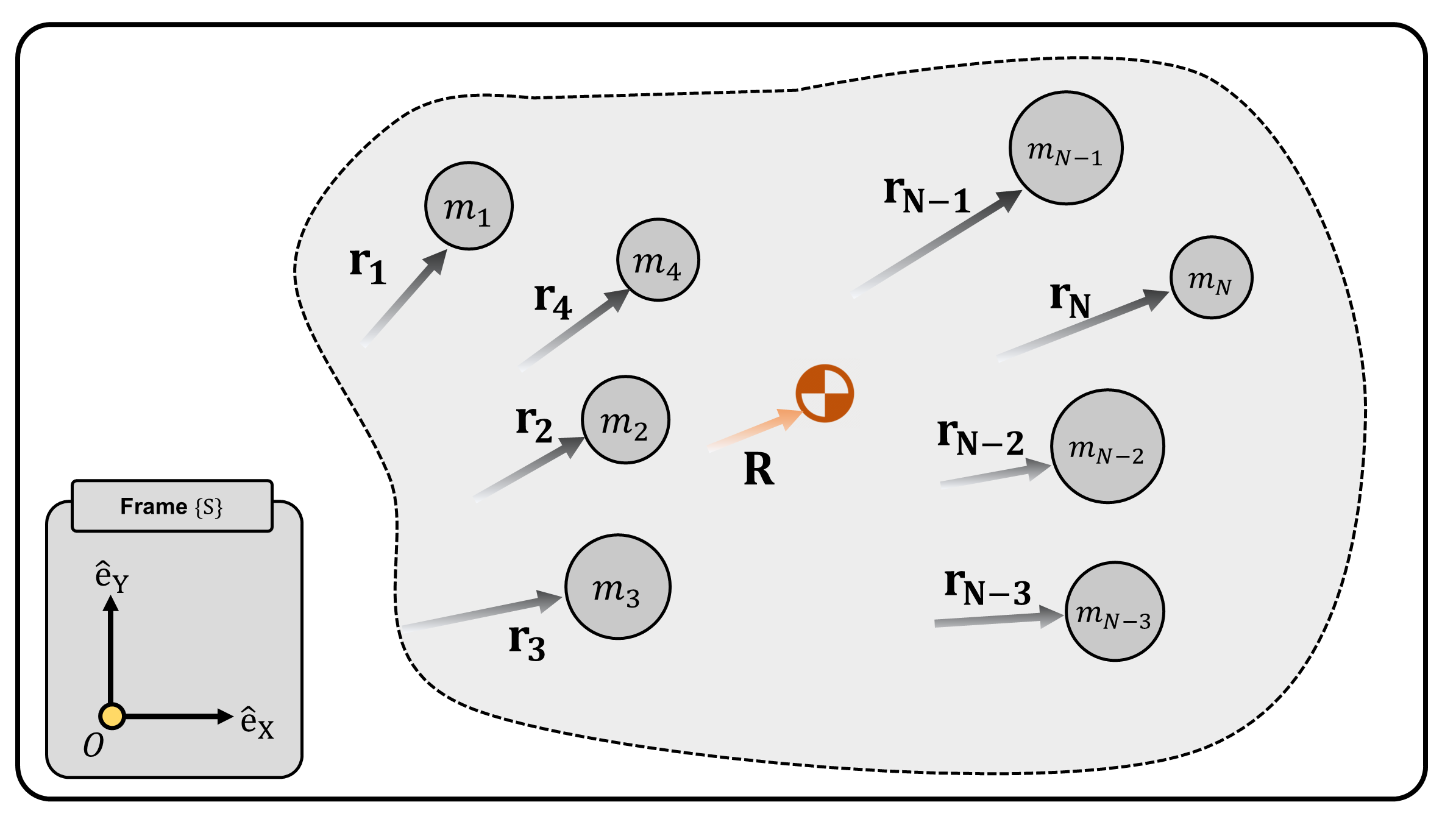
(Figure 1) A rigid object which consists of \(N\) particles and its center of mass \(\mathbf{R}\).
Center of Mass simplifies Euler’s First Law of Motion
The analysis of the motion of rigid objects can be simplified via the center of mass. We revisit Euler’s First Law of motion, i.e., the linear momentum principle of rigid objects: \[ \sum \mathbf{F}_{ext} = \frac{d\mathbf{P}}{dt} \] Let the center of mass and the total mass of the object be \(\mathbf{R}\) and \(M:=\sum m_i\), respectively. By definition, \(\mathbf{P}\) is simply: \[ \mathbf{P} := \sum_{i=1}^{N} m_i \mathbf{v}_i = M \cdot \frac{ \sum_{i=1}^{N}m_i\mathbf{v}_i}{M} = M \frac{d\mathbf{R}}{dt} \] Hence, Euler’s First Law of motion is reformulated as: \[ \sum \mathbf{F}_{ext} = M\frac{d^2\mathbf{R}}{dt^2} \] The result is simple yet elegant. No matter how complex the motion of the rigid object may be, there is a special point called the center of mass of the rigid object, which moves as if it is a point particle with mass \(M\) with all external forces applied to it (Figure 2A, 2B). We introduce a direct quote from Richard Feynman:
Newton’s law is also correct for large rigid objects, if we study not so much the details, but only the motion of the center of mass and the total external forces applied to the rigid object.
In other words, by focusing on the center of mass of the rigid object, Newton’s Laws of motion is reproduced in a larger scale!
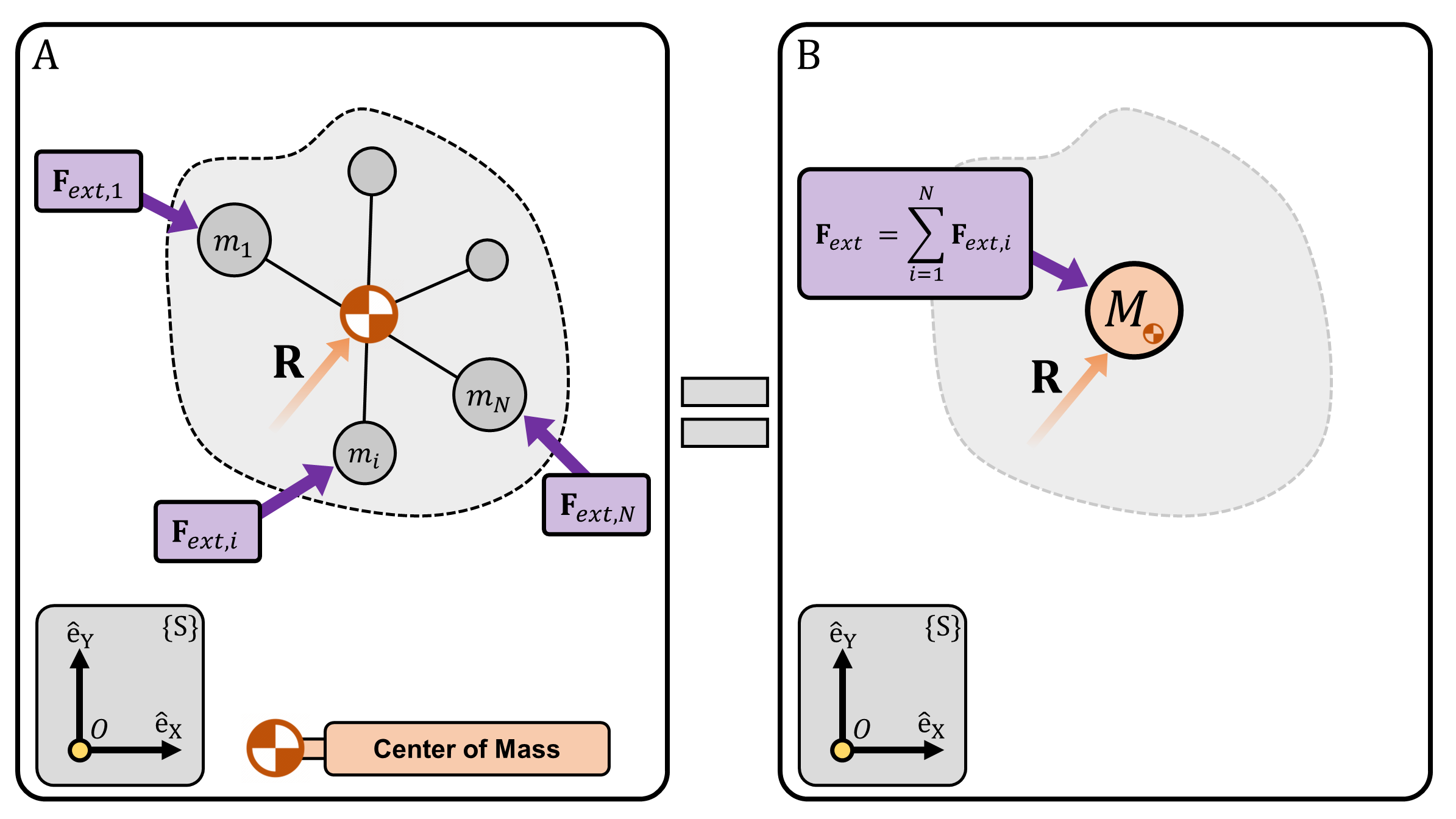
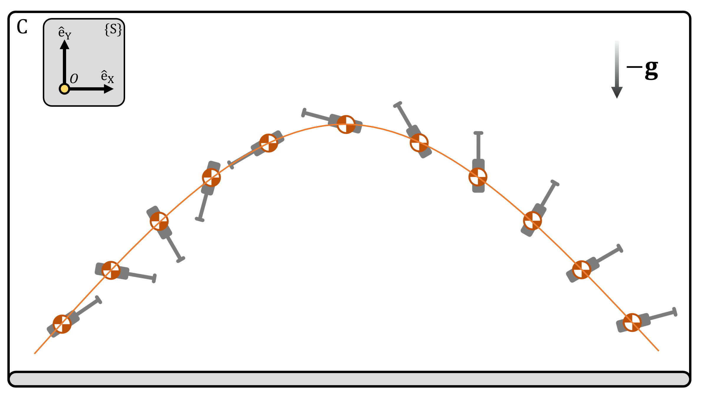
(Figure 2) (A) A collection of \(N\) particles with total mass \(M:=\sum m_i\). (B) The motion of the center of mass of (A) can be simplified as a single particle with mass \(M\) exerted by force \(\mathbf{F}_{ext}:=\sum\mathbf{F}_{ext,i}\). (C) No matter what the shape of the rigid object may be, if the object is thrown, under the influence of gravity, the center of mass of the object follows a parabola.