Angular Momentum Principle
Moses C. Nah
2023-03-06
Introduction
From the linear momentum principle, one can deduce the angular momentum principle for a single particle. For the angular momentum principle, we introduce two physical quantities — torque and angular momentum of a particle about some arbitrary point.
Angular Momentum and Torque of a Single Particle
Consider a particle with mass \(m\) (Figure 1). Force \(\mathbf{F}\) is applied to the particle. Given point \(O\), We define torque \(\boldsymbol{\tau}_O\) on a point particle about a fixed point \(O\) as: \[ \boldsymbol{\tau}_O := \mathbf{r} \times \mathbf{F} \tag{1} \] In this equation, \(\mathbf{r}\in\mathbb{R}^3\) is the position of the particle measured from a fixed point \(O\), Operator \(\times\) denotes the cross product between two vectors.1
Moreover, we define the angular momentum \(\mathbf{H}_O\) of the particle about point \(O\) as: \[ \mathbf{H}_O := \mathbf{r} \times \mathbf{p} \tag{2} \] In this equation, \(\mathbf{p}\in\mathbb{R}^3\) is the linear momentum of the particle.
Note that both, torque and angular momentum are defined with respect to a reference point. Meaning, both torque and angular momentum changes with respect to the choice of the reference point. To emphasize the point to which the torque and angular momentum are referenced, subscript is always (and must be) added to the torque and angular momentum. We later show that a careful choice of reference point to define torque and angular momentum can simplify the analysis of the motion.
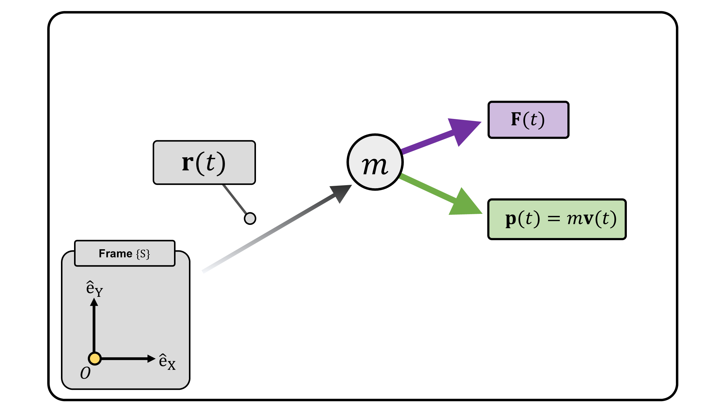
(Figure 1) A point particle with mass \(m\) moving with linear momentum \(\mathbf{p}=m\mathbf{v}\). \(O\) is the reference point.
Angular Momentum Principle
As with the linear momentum principle of \(\mathbf{F}=\dot{\mathbf{p}}\) from Newton’s second law of motion, one can derive the angular momentum principle, which shows the relation between torque and angular momentum about some reference point.
Consider the linear momentum principle of a single particle: \[ \mathbf{F} = \frac{d\mathbf{p}}{dt} \] Given a fixed reference point \(O\), we apply the cross product of \(\mathbf{r}\), which is the distance from \(O\) to the particle, on both sides of the equation: \[ \mathbf{r} \times F = \mathbf{r} \times \frac{d}{dt}\mathbf{p} \] A bit of math trick gives us: \[ \require{cancel} \boldsymbol{\tau}_O := \mathbf{r} \times F = \mathbf{r} \times \frac{d\mathbf{p}}{dt} = \frac{d}{dt} (\mathbf{r}\times \mathbf{p}) - \frac{d}{dt}\mathbf{r}\times \mathbf{p} = \frac{d\mathbf{H}_O}{dt} - \ \cancel{\mathbf{v}\times\mathbf{p}} = \frac{d\mathbf{H}_O}{dt} \] Note that \(\mathbf{p}=m\mathbf{v}\) is parallel to \(\mathbf{v}\), hence \(\mathbf{v}\times\mathbf{p}\) is zero.2
From the linear momentum principle, we derive the angular momentum principle of a particle about fixed point \(O\): \[ \boldsymbol{\tau}_O = \frac{d\mathbf{H}_O}{dt} \tag{3} \]
Angular momentum principle is reminiscent of the linear momentum principle. For instance, if the torque \(\boldsymbol{\tau}_O\) with respect to point \(O\) is zero, then the angular momentum \(\mathbf{H}_O\) about point \(O\) is conserved. This is the conservation of angular momentum. Hence, one can choose a reference point \(O\) which results in zero torque and use the conservation of angular momentum to simplify the analysis of the problem. For instance, one of the example problems in this post use the conservation of angular momentum to simplify the analysis.
Angular Momentum Principle about a General Point
The angular momentum principle of Equation 3 is derived with respect to a fixed reference point \(O\) (Figure 1). One can further generalize the angular momentum principle about a moving point \(A\). Consider another point \(A\) that can either be fixed or moving (Figure 2) The kinematic relation between point \(O\), point \(A\) and mass \(m\) is: \[ \mathbf{r} = \mathbf{r}_A + \mathbf{r}' \tag{4} \]
By definition, the torque and angular momentum of the particle about point \(A\) are: \[ \boldsymbol{\tau}_A := \mathbf{r}' \times \mathbf{F} ~~~~~~~~~~~~~ \mathbf{H}_A := \mathbf{r}' \times \mathbf{p} \] Taking the time derivative of \(\mathbf{H}_A\) gives us: \[ \require{cancel} \begin{align*} \frac{d\mathbf{H}_A}{dt} &:= \frac{d}{dt}(\mathbf{r'}\times\mathbf{p})= \frac{d}{dt}\mathbf{r}' \times \mathbf{p} + \mathbf{r}'\times \frac{d}{dt}\mathbf{p} = \frac{d}{dt}\underbrace{(\mathbf{r}-\mathbf{r}_A)}_{\text{Equation 4} }\times \mathbf{p}+\mathbf{r'}\times \mathbf{F} \\ &= ( \mathbf{v} - \mathbf{v}_A) \times \mathbf{p} +\mathbf{\tau}_A = \cancel{\mathbf{v\times p}} - \mathbf{v}_A\times\mathbf{p}+\boldsymbol{\tau}_A \end{align*} \]
We derive angular momentum principle about a general point \(A\): \[ \boldsymbol{\tau}_A = \frac{d\mathbf{H}_A}{dt} +\mathbf{v}_A\times \mathbf{p} \tag{5} \] It is immediate that Equation 3 is a special case of Equation 5 when \(A\) is stationary, i.e., \(\mathbf{v}_A = \mathbf{0}\).
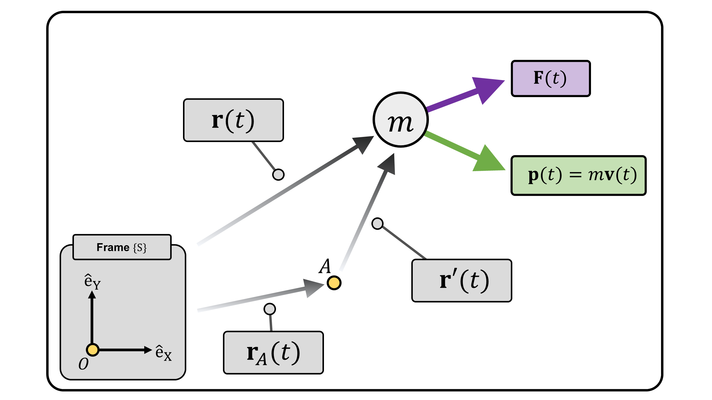
(Figure 2) A diagram modified from Figure 1 but with an additional point \(A\).
Examples
Several Examples are presented to solidify our understanding.
Example 1: A Rotating Mass
Consider a particle with mass \(m\) that is attached to a taut string (Figure 3). Due to the taut string with tension \(T\), the mass particle is rotating on a frictionless planar surface. A mass is initially rotating with radius \(r_1\) with velocity \(v_1\). Assume that one pulled down the string so that the radius changed from \(r_1\) to \(r_2\).
By a careful choice of reference point, this problem can be solved in a single line using the conservation of angular momentum. Since the tension force is always passing through point \(O\) (Figure 3, Right), the torque with respect to point \(O\) is zero. This implies that the angular momentum of the point mass \(m\) about point \(O\) is preserved.
Therefore, the angular momentum at radius \(r_1\) and \(r_2\) is identical: \[ mr_1v_1 = mr_2 v_2, \;\;\;\; v_2 =\frac{r_1}{r_2}v_1 \] Meaning, if the radius reduces to half, the speed is doubled. This example is in lieu of Kepler’s 2nd law of planatary motion.
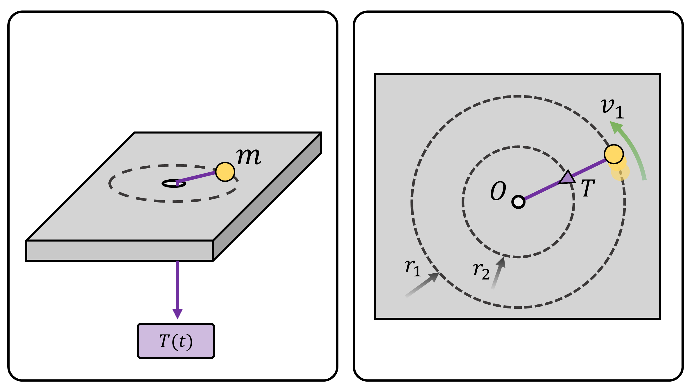
(Figure 3) (Left) A 3D view of a mass pulled from a string. The mass is sliding on a frictionless planar surface. (Right) A 2D planar view of the left image.
For people who are familiar with tensor calculus, we can concisely describe the cross product of two vectors using tensor notation. Consider two vectors \(\mathbf{a,b}\in\mathbb{R}^3\). The \(i\)-th component of \(\mathbf{a}\times \mathbf{b}\) is: \[ (\mathbf{a}\times \mathbf{b})_i = \epsilon_{ijk} a_j b_k \] where \(\epsilon\) denotes the Levi-Civita symbol. For instance, the components of \(\mathbf{a}\times\mathbf{b}\) are: \[ \begin{align} (\mathbf{a}\times \mathbf{b})_1 &= \epsilon_{1jk} a_j b_k = \epsilon_{123} a_2 b_3 + \epsilon_{132} a_3 b_2 = a_2b_3 - a_3b_2 \\ (\mathbf{a}\times \mathbf{b})_2 &= \epsilon_{2jk} a_j b_k = \epsilon_{213} a_1 b_3 + \epsilon_{231} a_3 b_1 = a_3b_1 - a_1b_3 \\ (\mathbf{a}\times \mathbf{b})_3 &= \epsilon_{3jk} a_j b_k = \epsilon_{312} a_1 b_2 + \epsilon_{321} a_2 b_1 = a_1b_2-a_2b_1 \\ \end{align} \] We can also describe this using the following matrix formulation: \[ \mathbf{a}\times\mathbf{b}= \begin{bmatrix} 0 & -a_3 & a_2 \\ a_3 & 0 & -a_1 \\ -a_2 & a_1 & 0 \end{bmatrix} \begin{bmatrix} b_1 \\ b_2 \\ b_3 \end{bmatrix} := [\mathbf{a}] \mathbf{b} \] where \([\cdot]:\mathbb{R}^3\rightarrow \mathbb{R^{3\times3} }\) is the operator that changes a 3D vector into its equivalent matrix as shown above. The operator will be often used throughout the posts. ↩︎
Again, a zero vector, not a zero scalar.↩︎