Exponential Coordinates of Rotation Matrix
Moses C. Nah
2023-06-09
Introduction
In the previous post, we show that rotation matrix \(\mathbf{R}\) is an element of a \(SO(3)\) group, and represents a rigid body transformation. Here, we bridge the relation between rotation matrix \(\mathbf{R}\) and the rotation about a unit axis \(\hat{\boldsymbol{\omega}}\) with angle \(\theta\).
Exponential Coordinates of Rotation Matrix
Consider \(\mathbf{p}\in\mathbb{R}^3\) which rotates about unit axis \(\hat{\boldsymbol{\omega}}\). We define a fixed, inertial frame \(\{S\}\) to describe the components of \(\mathbb{R}^3\), and for notational simplicity, we omit the superscript \(s\).
It is well-known that the velocity of \(\mathbf{p}\) is defined by (Figure 1, Left): \[ \dot{\mathbf{p}} = \hat{\boldsymbol{\omega}} \times \mathbf{p} \]
The cross product of \(\hat{\boldsymbol{\omega}}\) can be
expressed in matrix form: \[
\hat{\boldsymbol{\omega}}=
\begin{pmatrix}
\hat{\omega}_x \\
\hat{\omega}_y \\
\hat{\omega}_z
\end{pmatrix}
~~~~~~
[\hat{\boldsymbol{\omega}}]=
\begin{pmatrix}
0 & -\hat{\omega}_z & \hat{\omega}_y \\
\hat{\omega}_z & 0 & -\hat{\omega}_x \\
-\hat{\omega}_y & \hat{\omega}_x & 0
\end{pmatrix}
~~~~~~
\dot{\mathbf{p}} = [\hat{\boldsymbol{\omega}}]\mathbf{p}
\] The resulting equation is a first-order linear differential
equation of \(\dot{\mathbf{x}}=\mathbf{Ax}\) form. The
closed-form solution for this equation is well-known: \[
\mathbf{p}(t) = \exp([\hat{\boldsymbol{\omega}}]t) ~\mathbf{p}(0)
\] In this equation, \(\exp(\cdot):\mathbb{R}^{3\times 3}\rightarrow
\mathbb{R}^{3\times 3}\) is called the exponential
map defined by: \[
\exp([\hat{\boldsymbol{\omega}}]t) = \mathbf{I}_3 +
[\hat{\boldsymbol{\omega}}]t+\frac{1}{2!}[\hat{\boldsymbol{\omega}}]^2t^2
+ \cdots + \frac{1}{n!}[\hat{\boldsymbol{\omega}}]^nt^n +\cdots \tag{1}
\]
Here, we set \(\theta=t\), i.e., \(\mathbf{p}\) rotates at a constant rate of
1rad/s from \(t=0\) to \(t=\theta\). Hence, \(\exp([\hat{\boldsymbol{\omega}}]\theta)\)
transforms \(\mathbf{p}\) by rotating
it about \(\hat{\boldsymbol{\omega}}\)
with angle \(\theta\).
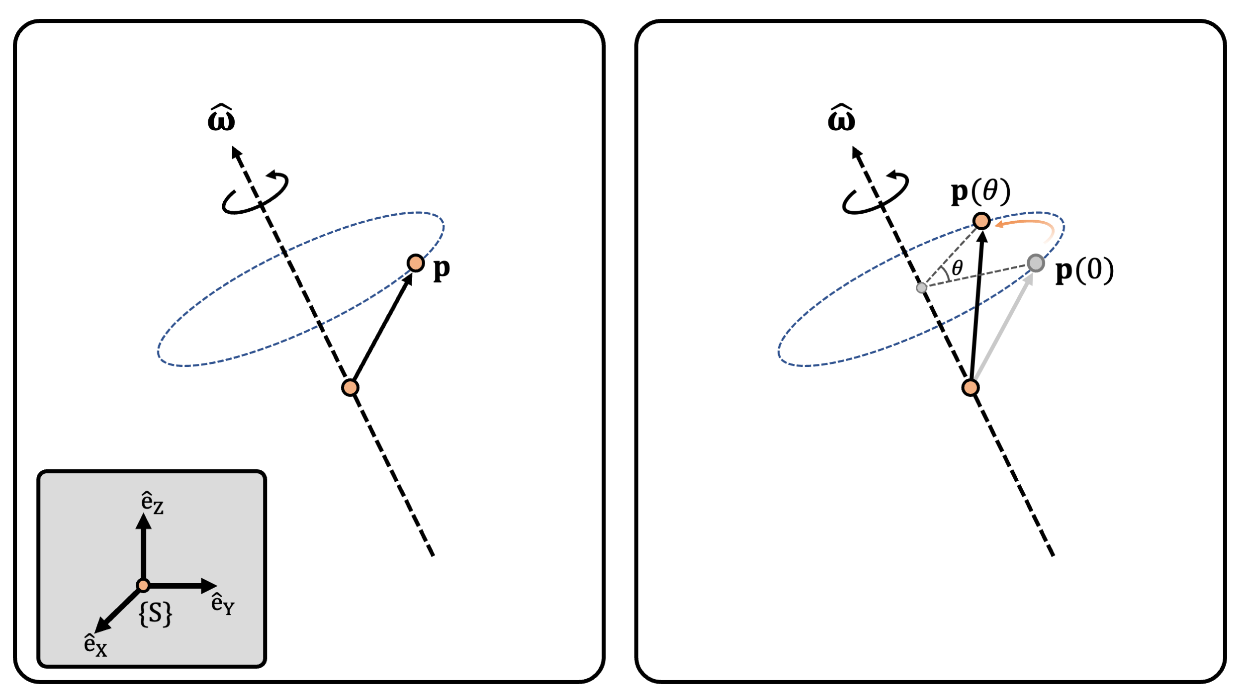
(Figure 1) (Left) Rotation of \(\mathbf{p}\) about unit axis \(\hat{\boldsymbol{\omega}}\). (Right) Rotation of \(\mathbf{p}\) about unit axis \(\hat{\boldsymbol{\omega}}\) with angle \(\theta\).
Since \([\hat{\boldsymbol{\omega}}]\) is a \(\mathbb{R}^{3\times 3}\) matrix, based on
Cayley-Hamilton
theorem, all the terms with order higher than 3 can be expressed as
a sum of \(\mathbf{I}_3,
[\hat{\boldsymbol{\omega}}], [\hat{\boldsymbol{\omega}}]^2\).
Based on the characteristic equation of \([\hat{\boldsymbol{\omega}}]\), we have:
\[
\det(\lambda\mathbf{I}-[\hat{\boldsymbol{\omega}}]) = \lambda^3 +
(\hat{\omega}_x^2+\hat{\omega}_y^2+\hat{\omega}_z^2)\lambda =
\lambda^3+\lambda ~~~~~~~~~~~~~~~
[\hat{\boldsymbol{\omega}}]^3=-[\hat{\boldsymbol{\omega}}]
\] The infinite sum of Equation 1 can be simplified: \[
\begin{align*}
\exp([\hat{\boldsymbol{\omega}}]\theta) &= \mathbf{I}_3 +
[\hat{\boldsymbol{\omega}}]\theta+\frac{1}{2!}[\hat{\boldsymbol{\omega}}]^2\theta^2
+ \cdots + \frac{1}{n!}[\hat{\boldsymbol{\omega}}]^n\theta^n +\cdots \\
&= \mathbf{I}_3 + [\hat{\boldsymbol{\omega}}]\theta +
\frac{1}{2!}[\hat{\boldsymbol{\omega}}]^2\theta^2 -
\frac{1}{3!}[\hat{\boldsymbol{\omega}}]\theta^3 -
\frac{1}{4!}[\hat{\boldsymbol{\omega}}]^2\theta^2+ \cdots \\
&= \mathbf{I}_3 +
[\hat{\boldsymbol{\omega}}]\Big(\theta-\frac{1}{3!}\theta^3+\cdots\Big)
+ [\hat{\boldsymbol{\omega}}]^2\Big(
\frac{\theta^2}{2!}-\frac{\theta^4}{4!}+\cdots \Big) \\
&= \mathbf{I}_3 + \sin\theta[\hat{\boldsymbol{\omega}}] +
(1-\cos\theta)[\hat{\boldsymbol{\omega}}]^2
\end{align*}
\] This is the famous Rodrigues’
rotation formula: \[
\exp([\hat{\boldsymbol{\omega}}]\theta)= \mathbf{I}_3 +
\sin\theta[\hat{\boldsymbol{\omega}}] +
(1-\cos\theta)[\hat{\boldsymbol{\omega}}]^2 \tag{2}
\]
Rodrigues’ Rotation Formula
In fact, the more well-known Rodrigues’ formula is as follows: \[ \mathbf{v}' = \mathbf{v}\cos\theta + (\hat{\boldsymbol{\omega}}\times\mathbf{v})\sin\theta + \hat{\boldsymbol{\omega}}(\hat{\boldsymbol{\omega}} \cdot \mathbf{v})(1-\cos\theta) \tag{3} \] In this equation, \(\mathbf{v}\) is mapped to \(\mathbf{v}'\) by rotating \(\mathbf{v}\) about unit axis \([\hat{\boldsymbol{\omega}}]\) with angle \(\theta\). We show that Equation 3 can be derived from Equation 2. Before that, we introduce the following identity:1 \[ [\hat{\boldsymbol{\omega}}]^2 = \hat{\boldsymbol{\omega}}\hat{\boldsymbol{\omega}}^{\mathbf{T}}-||\hat{\boldsymbol{\omega}}||^2\mathbf{I}_3 = \hat{\boldsymbol{\omega}}\hat{\boldsymbol{\omega}}^{\mathbf{T}}-\mathbf{I}_3 \] Multiplying Equation 2 with \(\mathbf{v}\in\mathbb{R}^3\) results in Equation 3: \[ \begin{align*} \exp([\hat{\boldsymbol{\omega}}]\theta) \mathbf{v} &= \mathbf{v}+ \sin\theta[\hat{\boldsymbol{\omega}}]\mathbf{v} + (1-\cos\theta)[\hat{\boldsymbol{\omega}}]^2 \mathbf{v} = \mathbf{v} + (\hat{\boldsymbol{\omega}} \times \mathbf{v})\sin\theta + (1-\cos\theta)( \hat{\boldsymbol{\omega}}\hat{\boldsymbol{\omega}}^{\mathbf{T}}\mathbf{v} - \mathbf{v} ) \\ &= \cos\theta \mathbf{v}+(\hat{\boldsymbol{\omega}} \times \mathbf{v})\sin\theta + \hat{\boldsymbol{\omega}}(\hat{\boldsymbol{\omega}}\cdot\mathbf{v})(1-\cos\theta) \end{align*} \]
A Quick Example
Consider we rotate \(\mathbf{p}\) about the unit \(\mathrm{\hat{e}_Z}\) axis with angle \(\theta\). Then, \(\hat{\boldsymbol{\omega}}=(0,0,1)\), and by definition: \[ [\hat{\boldsymbol{\omega}}]= \begin{pmatrix} 0 & -\hat{\omega}_z & \hat{\omega}_y \\ \hat{\omega}_z & 0 & -\hat{\omega}_x \\ -\hat{\omega}_y & \hat{\omega}_x & 0 \end{pmatrix} = \begin{pmatrix} 0 & -1 & 0 \\ 1 & 0 & 0 \\ 0 & 0 & 0 \end{pmatrix} ~~~~~~~~ [\hat{\boldsymbol{\omega}}]^2 = \begin{pmatrix} -1 & 0 & 0 \\ 0 & -1 & 0 \\ 0 & 0 & 0 \end{pmatrix} \] Using the Rodrigues’ formula: \[ \exp([\hat{\boldsymbol{\omega}}]\theta)= \mathbf{I}_3 + \sin\theta \begin{pmatrix} 0 & -1 & 0 \\ 1 & 0 & 0 \\ 0 & 0 & 0 \end{pmatrix} + (1-\cos\theta) \begin{pmatrix} -1 & 0 & 0 \\ 0 & -1 & 0 \\ 0 & 0 & 0 \end{pmatrix} = \begin{pmatrix} \cos\theta & -\sin\theta & 0 \\ \sin\theta & \phantom{-}\cos\theta & 0 \\ 0 & 0 & 1 \end{pmatrix} \] The result is the well-known form.
The Exponential Map is Surjective onto SO(3) [1]
We show that \(\exp([\hat{\boldsymbol{\omega}}]\theta)\) is an element of Special Orthogonal group, SO(3). The proof is straightforward, since all we need to check is (1) \(\exp([\hat{\boldsymbol{\omega}}]\theta)\) is an orthogonal matrix and (2) determinant value of \(\exp([\hat{\boldsymbol{\omega}}]\theta)\) is 1.
Proof 1
Based on Rodrigues’ formula (Equation 2), the transpose of \(\exp([\hat{\boldsymbol{\omega}}]\theta)\) is: \[ \exp([\hat{\boldsymbol{\omega}}]\theta)^{\textbf{T}} = \mathbf{I}_3 - \sin\theta [\hat{\boldsymbol{\omega}}] + (1-\cos\theta)[\hat{\boldsymbol{\omega}}]^2 = \exp(-[\hat{\boldsymbol{\omega}}]\theta) \] If we simply multiply \(\exp([\hat{\boldsymbol{\omega}}]\theta)\) with \(\exp([\hat{\boldsymbol{\omega}}]\theta)^{\textbf{T}}\), and use Cayley-Hamilton’s theorem: \[ \begin{align*} \exp([\hat{\boldsymbol{\omega}}]\theta) \exp([\hat{\boldsymbol{\omega}}]\theta)^{\textbf{T}} &= \{ \mathbf{I}_3 - \sin\theta [\hat{\boldsymbol{\omega}}] + (1-\cos\theta)[\hat{\boldsymbol{\omega}}]^2 \} \{ \mathbf{I}_3 + \sin\theta [\hat{\boldsymbol{\omega}}] + (1-\cos\theta)[\hat{\boldsymbol{\omega}}]^2 \} \\ &= \mathbf{I}_3 + [\hat{\boldsymbol{\omega}}]^2( 2-2\cos\theta-\sin^2\theta ) + [\hat{\boldsymbol{\omega}}]^4(1-\cos\theta)^2 = \mathbf{I}_3 \end{align*} \]
Proof 2
Using Jacobi’s formula: \[ \det( \exp([\hat{\boldsymbol{\omega}}]\theta) ) = \exp( ~ \text{tr}( [\hat{\boldsymbol{\omega}}]\theta ) ~ ) = \exp( 0 ) = 1 \] Hence, \(\exp([\hat{\boldsymbol{\omega}}]\theta)\) is an element of \(SO(3)\) group.
Some Properties
Based on Rodrigues’ formula (Equation 2), we can show some major properties of \(\exp([\hat{\boldsymbol{\omega}}]\theta)\). We leave it as an exercise to the readers:
- (Property 1) \[ \{ \exp([\hat{\boldsymbol{\omega}}]\theta) \}^{\text{T}} = \exp([\hat{\boldsymbol{\omega}}]^{\text{T}}\theta) = \exp(-[\hat{\boldsymbol{\omega}}]\theta) = \{ \exp([\hat{\boldsymbol{\omega}}]\theta) \}^{-1} \tag{P1} \]
- (Property 2) \[ [\hat{\boldsymbol{\omega}}]\exp([\hat{\boldsymbol{\omega}}]\theta) = \exp([\hat{\boldsymbol{\omega}}]\theta)[\hat{\boldsymbol{\omega}}] \tag{P2} \]
References
Note that this equation appears when we define the moment of inertia of a rigid object↩︎