The Cart and Pendulum
Moses C. Nah
2023-02-13
We analyze the kinematics and dynamics of the famous Cart and Pendulum. This will be a good example problem to apply the theories which have been presented. Consider the cart and pendulum system shown in Figure 1. Our goal is to find the equations of motion of this system. Since there are two degrees of freedom described with coordinates \(x\) and \(\theta\), we expect to have two differential equations for the equations of motion.
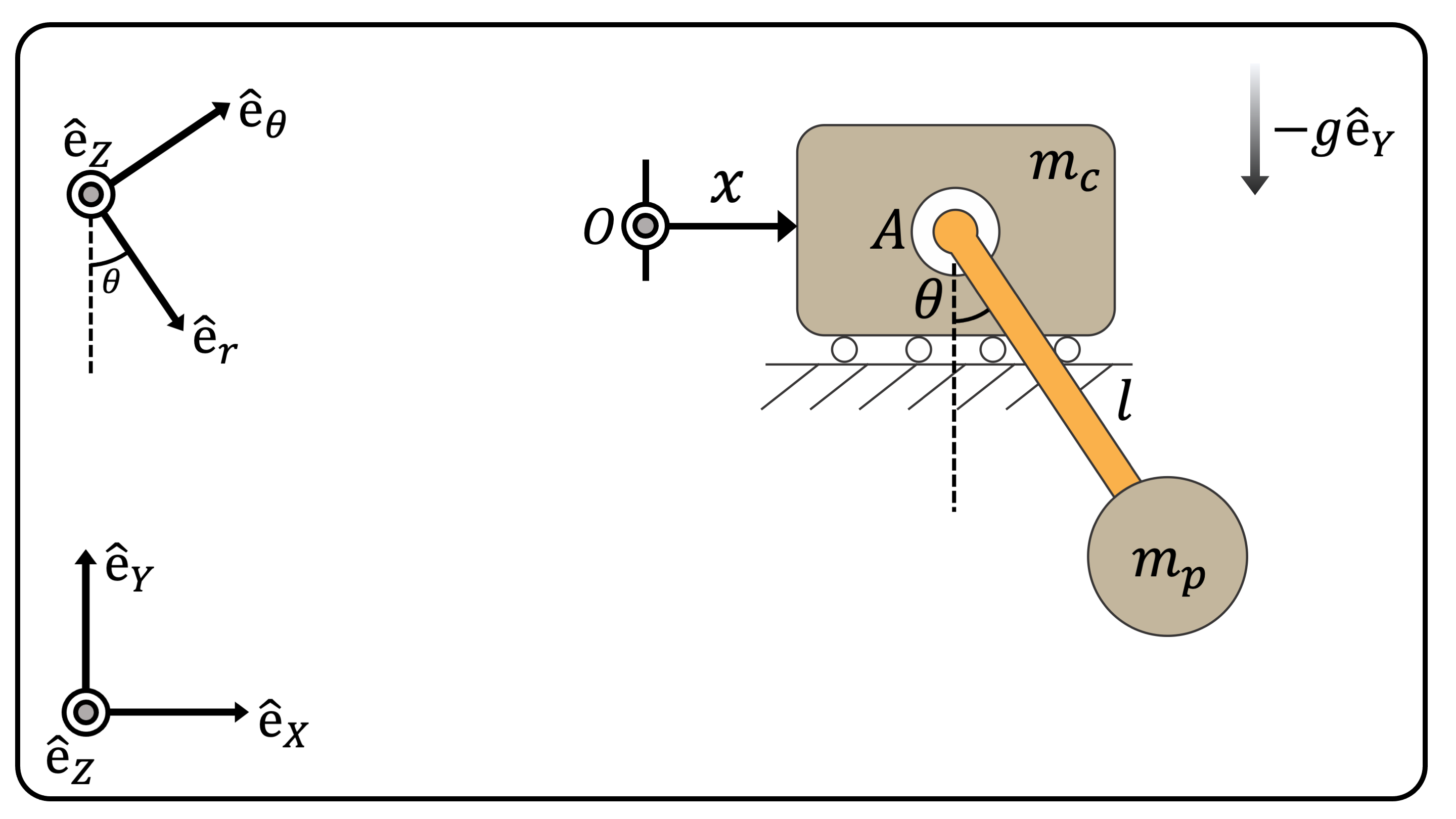
(Figure 1) The Cart and Pendulum. \(O\) is the origin of the system.
Kinematics
The position, velocity and acceleration of the cart, \(\mathbf{r}_C\), \(\mathbf{v}_C\), \(\mathbf{a}_C\), are: \[ \begin{align} \mathbf{r}_C &= x \hat{e}_X \\ \mathbf{v}_C &= \dot{x} \hat{e}_X \\ \mathbf{a}_C &= \ddot{x} \hat{e}_X \end{align} \] Note that the orthonormal basis vectors \(\hat{e}_X\), \(\hat{e}_Y\), \(\hat{e}_Z\) are fixed, hence not considered for the time derivative.
The position, velocity and acceleration of the point mass attached at the end of the pendulum, \(\mathbf{r}_P\), \(\mathbf{v}_P\), \(\mathbf{a}_P\), are:
\[ \begin{align} \mathbf{r}_P &= (x + l\sin\theta ) \hat{e}_X - ( l \cos\theta)\hat{e}_Y \\ \mathbf{v}_P &= (\dot{x} + l\dot{\theta}\cos\theta )\hat{e}_X + l\dot{\theta}\sin\theta \hat{e}_Y \\ \mathbf{a}_P &= (\ddot{x}+l\ddot{\theta}\cos\theta - l\dot{\theta}^2\sin\theta)\hat{e}_X + (l\ddot{\theta}\sin\theta + l\dot{\theta}^2\cos\theta)\hat{e}_Y \end{align} \] Another way to derive the kinematics of the pendulum is to define a rotating orthonormal basis vectors, \(\hat{e}_r\), \(\hat{e}_\theta\):
\[ \begin{align} \hat{e}_r &= \sin\theta \hat{e}_X - \cos\theta \hat{e}_Y \;\;\;\; \dot{\hat{e}}_r = \dot{\theta}\cos\theta\hat{e}_X + \dot{\theta}\sin\theta\hat{e}_Y = \dot{\theta} \hat{e}_\theta \\ \hat{e}_\theta &= \cos\theta \hat{e}_X + \sin\theta \hat{e}_Y \;\;\;\; \dot{\hat{e}}_\theta = -\dot{\theta}\sin\theta \hat{e}_X + \dot{\theta}\cos\theta \hat{e}_Y = -\dot{\theta}\hat{e}_r \\ \end{align} \] And therefore, \[ \begin{align} \mathbf{r}_P &= x \hat{e}_X + l\hat{e}_r = (x + l\sin\theta)\hat{e}_X - l\cos\theta\hat{e}_Y \\ \mathbf{v}_P &= \dot{x}\hat{e}_X + l\dot{\hat{e}}_r = \dot{x}\hat{e}_X + l\dot{\theta}\hat{e}_\theta = ( \dot{x} + l\dot{\theta}\cos\theta)\hat{e}_X + l\dot{\theta}\sin\theta\hat{e}_Y \\ \mathbf{a}_P &= \ddot{x}\hat{e}_X + l\ddot{\theta}\hat{e}_\theta + l\dot{\theta}\dot{\hat{e}}_\theta = \ddot{x}\hat{e}_X + l\ddot{\theta}\hat{e}_\theta - l\dot{\theta}^2\hat{e}_r = ( \ddot{x} + l\ddot{\theta}\cos\theta - l\dot{\theta}^2\sin\theta)\hat{e}_X + (l\ddot{\theta}\sin\theta + l\dot{\theta}^2\cos\theta)\hat{e}_Y \end{align} \]
The Free-body Diagram
The free-body diagram of the system is shown in Figure 2.
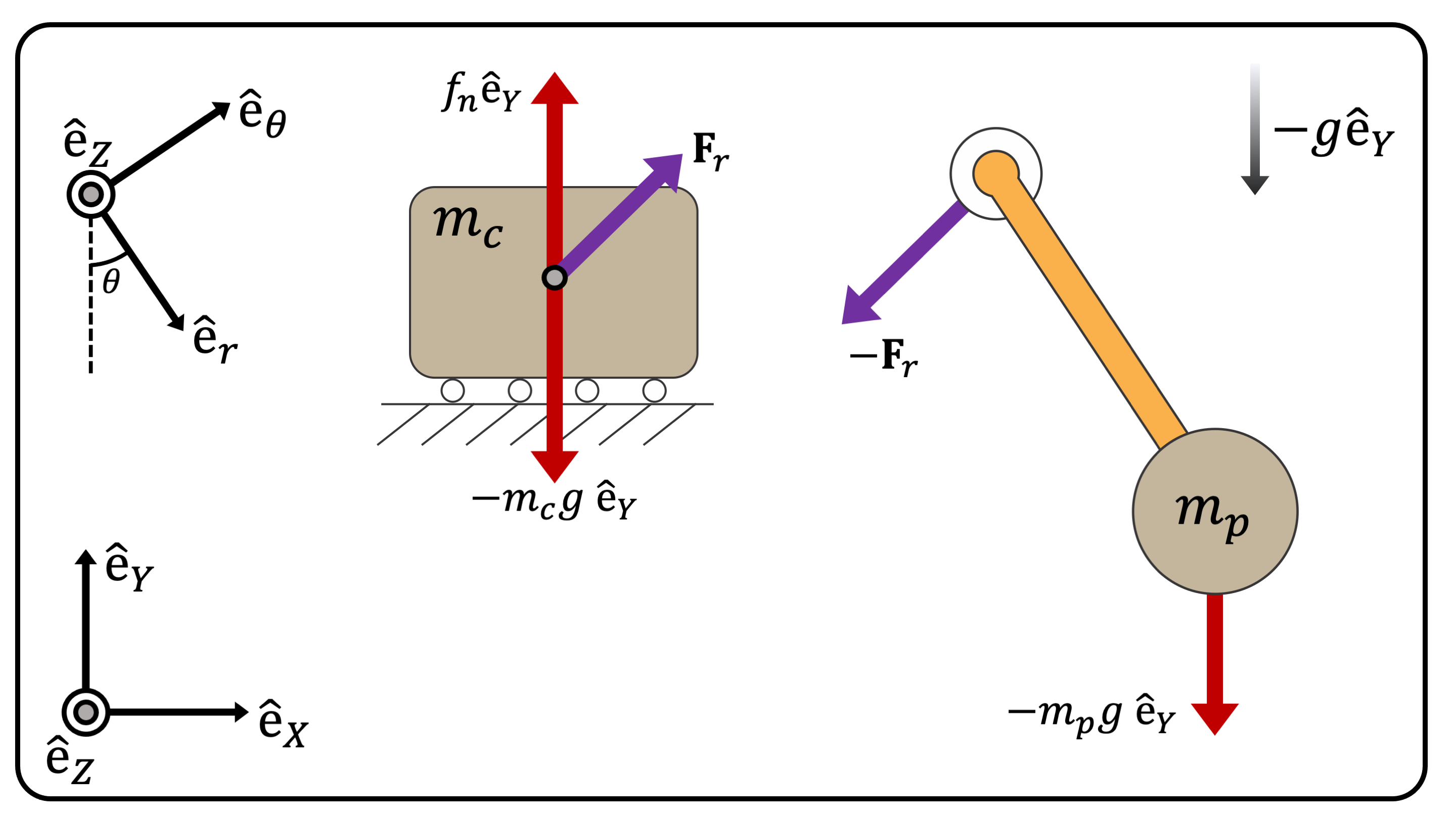
(Figure 2) The Free-body Diagram of the Cart and Pendulum
In detail:
- Force \(f_n \hat{e}_Y\) is the normal force of the cart which constrains the cart to move horizontally.
- Force \(\mathbf{F}_r\) is the interaction force between the cart and the pendulum. Based on Newton’s Third Law of Motion (i.e., the Law of Action and Reaction), the force vector \(\mathbf{F}_r\) applied to the pendulum is an equal and opposite reaction force of \(\mathbf{F}_r\) applied to the cart.
The Linear Momentum Principle
Based on the free-body diagram, we can apply the linear momentum principle to the cart and pendulum: \[ \begin{align} m_c \mathbf{a}_c &= \mathbf{F}_r + f_n\hat{e}_Y - m_cg\hat{e}_Y \\ m_p \mathbf{a}_p &= -\mathbf{F}_r - m_pg\hat{e}_Y \end{align} \] If we account for the Newton’s Third Law of Motion, we can discard the interaction force \(\mathbf{F}_r\) by adding the two equations:
\[ \begin{equation} m_c \mathbf{a}_c + m_p\mathbf{a}_p = \{ f_n-(m_c+m_p)g \}\hat{e}_Y \end{equation} \] The left hand-side of the equation is the time derivative of the total linear momentum of the system. Since the right hand-side of the equation shows that the total force applied to the whole system is only along the \(\hat{e}_Y\) axis, we show that the total linear momentum of the system along the \(\hat{e}_X\) axis is preserved: \[ \begin{equation} ( m_c \mathbf{a}_c + m_p\mathbf{a}_p ) \cdot \hat{e}_X = \{ f_n-(m_c+m_p)g \} (\hat{e}_Y \cdot \hat{e}_X ) = 0 \end{equation} \] Hence, we derive the first equation of motion of the system: \[ \begin{equation} (m_c + m_p) \ddot{x} +m_pl\ddot{\theta}\cos\theta - m_pl\dot{\theta}^2\sin\theta = 0 \tag{1} \end{equation} \]
The Angular Momentum Principle About Point A
To derive the second equation of motion, we use the angular momentum principle about point \(A\) (Figure 1). We derived the following equation at this post: \[ \tau_A = \frac{d}{dt}\mathbf{H}_A +\mathbf{v}_A\times \mathbf{p} \] The velocity of point \(A\) is simply the cart velocity \(\mathbf{v}_P\), \(\mathbf{v}_A = \mathbf{v}_P\).
The torque about point \(A\), \(\tau_A\), is: \[ \tau_A = (\mathbf{r}_P -\mathbf{r}_C ) \times (-m_p g)\hat{e}_Y = ( l\sin\theta\hat{e}_X - l\cos\theta \hat{e}_Y) \times (-m_p g)\hat{e}_Y = -m_pgl\sin\theta \hat{e}_Z \]
The angular momentum about point \(A\), \(\mathbf{H}_A\), is: \[ \begin{align} \mathbf{H}_A &= (\mathbf{r}_P -\mathbf{r}_C ) \times ( m_p \mathbf{v}_p ) = ( l\sin\theta\hat{e}_X - l\cos\theta \hat{e}_Y) \times \{ (m_p\dot{x} + m_pl\dot{\theta}\cos\theta )\hat{e}_X + m_pl\dot{\theta}\sin\theta \hat{e}_Y \} \\ &= ( m_p l^2 \dot{\theta}\sin^2\theta + m_pl\dot{x}\cos\theta + m_p l^2\dot{\theta}\cos^2\theta )\hat{e}_Z = (m_p l^2\dot{\theta} + m_pl\dot{x}\cos\theta)\hat{e}_Z \end{align} \] The time derivative of \(\mathbf{H}_A\) is: \[ \frac{d}{dt}\mathbf{H}_A = (m_p l^2 \ddot{\theta} + m_p l \ddot{x}\cos\theta - m_p l\dot{x}\dot{\theta}\sin\theta)\hat{e}_Z \] And: \[ \mathbf{v}_A \times \mathbf{p} = \dot{x} \hat{e}_X \times (m_p\mathbf{v}_p)= \dot{x}\hat{e}_X \times \{ (m_p\dot{x} + m_pl\dot{\theta}\cos\theta )\hat{e}_X + m_pl\dot{\theta}\sin\theta \hat{e}_Y \} = m_p l \dot{\theta}\dot{x}\sin\theta\hat{e}_Z \] Collecting all the terms, we have: \[ -m_pgl\sin\theta \hat{e}_Z = (m_p l^2 \ddot{\theta} + m_p l \ddot{x}\cos\theta - m_p l\dot{x}\dot{\theta}\sin\theta)\hat{e}_Z + m_p l \dot{\theta}\dot{x}\sin\theta\hat{e}_Z = (m_p l^2 \ddot{\theta} + m_p l \ddot{x}\cos\theta) \hat{e}_Z \] And we have derived the second equation of motion:
\[ m_p l^2 \ddot{\theta} + m_p l \ddot{x}\cos\theta + m_pgl\sin\theta = 0 \tag{2} \]
We can the answer is correct from this wonderful website made by Prof. Russ Tedrake from MIT.
The intuitive (but a bit hand-wavy) solution to derive the second equation of motion is to use the fictitious inertial force with respect to the frame \(A\) (Figure 3).
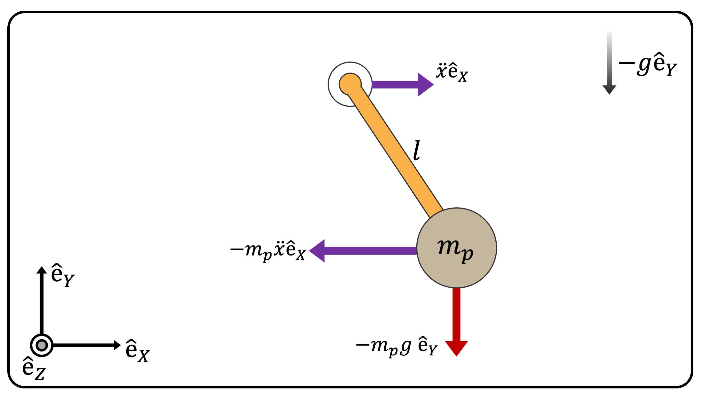
(Figure 3) The fictitious inertial force applied to the mass \(m_p\)
Hence, applying the torque equation about point \(A\) is: \[
m_p l^2 \ddot{\theta} = -m_p \ddot{x} l \cos\theta - m_pg l\sin\theta
\] which is the result that we have derived at Eq. (2).
The Equations of Motion
The Equations of motion of the cart and pendulum system are as follows: \[ \begin{align} (m_c + m_p) \ddot{x} +m_pl\ddot{\theta}\cos\theta - m_pl\dot{\theta}^2\sin\theta &= 0 \\ m_p l^2 \ddot{\theta} + m_p l \ddot{x}\cos\theta + m_pgl\sin\theta &= 0 \end{align} \]