First-order Joint-space Impedance Controller
Moses C. Nah
2023-12-01
Introduction
In this post, we introduce the first-order joint-space impedance controller, which can be considered as one of the most simple impedance controllers available.
As always, we consider an \(n\) degrees of freedom open-chain torque-actuated robot manipulator, where the dynamics is governed by the following equations of motion: \[ \forall t\ge 0: \mathbf{M}(\mathbf{q}(t))\ddot{\mathbf{q}}(t) + \mathbf{C}(\mathbf{q}(t), \dot{\mathbf{q}}(t))\dot{\mathbf{q}}(t) + \mathbf{g}(\mathbf{q}(t))=\boldsymbol{\tau}_\text{in}(t) \tag{1} \] The notations of the equation are self-explanatory, and we assume there are no external forces applied to the robot. Throughout this post, we assume that gravitational force vector \(\mathbf{g}(\mathbf{q}(t))\), is compensated, i.e., the \(\mathbf{g}(\mathbf{q}(t))\) term is neglected.
First-order Joint-space Impedance Controller
Given a proprioceptive feedback, i.e., \(\mathbf{q}(t)\) and \(\dot{\mathbf{q}}(t)\) are given, the first-order joint-space impedance controller is defined by: \[ \boldsymbol{\tau}_\text{in}(t) = \mathbf{Z}_{q}(\mathbf{q}(t), \mathbf{q}_0(t))= \mathbf{K}_q(\mathbf{q}_0(t)-\mathbf{q}(t)) + \mathbf{B}_q (\dot{\mathbf{q}}_0(t)-\dot{\mathbf{q}}(t))\tag{2} \] In this equation, \(\mathbf{K}_q,\mathbf{B}_q \in \mathbb{R}^{n\times n}\) are the joint stiffness and damping matrices; \(\mathbf{q}_0(t)\) is the virtual trajectory to which the (virtual joint) stiffness and damping are connected.
Stability Proof
If \(\mathbf{K_q},\mathbf{B_q}\) are chosen to be constant symmetric positive-definite matrices, for discrete joint-space movements, i.e., \(\exists T>0: \dot{\mathbf{q}}_0(t)=\mathbf{0}\) for \(t\ge T\), the first-order joint-space impedance controller has favorable stability property [2].
By setting \(\boldsymbol{\tau}_\text{in}(t)\) as the first-order joint-space impedance controller, the closed-loop dynamics is defined by: \[ \mathbf{M}(\mathbf{q}(t))\ddot{\mathbf{q}}(t) + \{ \mathbf{C}(\mathbf{q}(t), \dot{\mathbf{q}}(t)) + \mathbf{B}_{q} \}\dot{\mathbf{q}}(t) + \mathbf{K}_{q}(\mathbf{q}(t)-\mathbf{q}_0(t)) = \mathbf{0} \]
We define the following scalar function \(V(\mathbf{q}(t), \dot{\mathbf{q}}(t))\): \[ V(\mathbf{q}(t), \dot{\mathbf{q}}(t)) = \frac{1}{2}\dot{\mathbf{q}}(t)^{\top}\mathbf{M}(\mathbf{q}(t))\dot{\mathbf{q}}(t) + \frac{1}{2} \{\mathbf{q}(t)-\mathbf{q}_0(t)\}^{\top}\mathbf{K}_{q} \{\mathbf{q}(t)-\mathbf{q}_0(t)\} \] The physical meaning of the scalar function \(V(\mathbf{q}, \mathbf{\dot{q}})\) is the sum of kinetic and (virtual) elastic energy of the manipulator.
The time derivative of \(V(\mathbf{q}(t), \dot{\mathbf{q}}(t))\) is: \[ \require{cancel} \begin{align*} \frac{d}{dt}V(\mathbf{q}(t), \dot{\mathbf{q}}(t)) &= \dot{\mathbf{q}}(t)^{\top}\mathbf{M}(\mathbf{q}(t))\ddot{\mathbf{q}}(t) + \frac{1}{2}\dot{\mathbf{q}}(t)^{\top}\bigg( \frac{d}{dt}\mathbf{M}(\mathbf{q}(t)) \bigg) \dot{\mathbf{q}}(t) + \dot{\mathbf{q}}(t)^{\top}\mathbf{K}_{q}\{\mathbf{q}(t)-\mathbf{q}_0(t)\} \\ &= \cancel{ \dot{\mathbf{q}}(t)^{\top} \bigg( \frac{1}{2}\frac{d}{dt}\mathbf{M}(\mathbf{q}(t)) - \mathbf{C}(\mathbf{q}(t), \dot{\mathbf{q}}(t)) \bigg)\dot{\mathbf{q}}(t) } - \dot{\mathbf{q}}(t)^{\top}\mathbf{B}_{q}\dot{\mathbf{q}}(t) \le 0 \end{align*} \] Note that we used the well-known property in robotics [3], Property 2.6 of [4], where for all \(\mathbf{q}(t), \dot{\mathbf{q}}(t)\): \[ \forall \mathbf{v}\in\mathbb{R}^{n}: \mathbf{v}^{\top} \Big\{ \frac{1}{2}\frac{d}{dt}\mathbf{M}(\mathbf{q}(t)) - \mathbf{C}(\mathbf{q}(t), \dot{\mathbf{q}}(t)) \Big\} \mathbf{v}=0 \] \(\frac{d}{dt}V(\mathbf{q}(t), \dot{\mathbf{q}}(t))\) is negative semi-definite. Hence, we cannot directly use Lyapunov’s Global Stability Theorem [5]. Instead, we use LaSalle’s Global Invariant Set Theorem [7]. It is quick to check the following conditions. \[ \begin{align*} &(1)~~ \forall \mathbf{q}(t), \dot{\mathbf{q}}(t)\in\mathbb{R}^n: V(\mathbf{q}(t), \dot{\mathbf{q}}(t))>0 \\ &(2)~~ \forall \mathbf{q}(t), \dot{\mathbf{q}}(t)\in\mathbb{R}^n: \frac{d}{dt}V(\mathbf{q}(t), \dot{\mathbf{q}}(t)) \le 0 \\ &(3)~~ V(\mathbf{q}(t), \dot{\mathbf{q}}(t))\rightarrow \infty ~~ \text{as} ~~ ||(\mathbf{q}(t),\dot{\mathbf{q}}(t))||\rightarrow \infty: \text{Radial Unboundedness} \end{align*} \] Hence, \(\frac{d}{dt}V(\mathbf{q}(t), \dot{\mathbf{q}}(t))\rightarrow 0\) as \(t\rightarrow \infty\). Since \(\mathbf{B}_q\) is a positive-definite matrix, this implies \(\dot{\mathbf{q}}(t)\rightarrow \mathbf{0}\). And within the set of \(\dot{\mathbf{q}}(t)=\mathbf{0}\), the state converges to the largest invariant set, which is \(\mathbf{q}(t) \rightarrow \mathbf{q}_0\).
Stability Proof using Hamiltonian
One can also show the stability proof using Hamiltonian [1]. The Hamiltonian function \(\mathcal{H}(\mathbf{q}(t),\dot{\mathbf{p}}(t))\) of the Robotic manipulator is simply the total energy of the system: \[ \mathcal{H}(\mathbf{q}(t),\mathbf{p}(t)) = T(\mathbf{q}(t),\mathbf{p}(t))+V_g(\mathbf{q}(t)) = \frac{1}{2} \mathbf{p}(t)^{\top} \mathbf{M}(\mathbf{q}(t))^{-1}\mathbf{p}(t) + V_g(\mathbf{q}(t)) \] In this equation, \(V_g(\mathbf{q}(t))\) is the gravitational potential energy.
The Hamiltonian mechanics produces \(2n\) first-order differential equations: \[ \begin{align} \dot{\mathbf{q}}(t) &= \phantom{-}\frac{\partial \mathcal{H}(\mathbf{q}(t),\mathbf{p}(t))}{\partial \mathbf{p}} = \mathbf{M}^{-1}(\mathbf{q}(t))\mathbf{p}(t) \\ \dot{\mathbf{p}}(t) &= -\frac{\partial \mathcal{H}(\mathbf{q}(t),\mathbf{p}(t))}{\partial \mathbf{q}} + \boldsymbol{\tau}_{in}(t) = -\frac{\partial T(\mathbf{q}(t),\mathbf{p}(t))}{\partial \mathbf{q}} - \frac{\partial V_g(\mathbf{q}(t))}{\partial \mathbf{q}} + \boldsymbol{\tau}_{in}(t) \end{align} \] Note that \(\frac{\partial V_g(\mathbf{q}(t))}{\partial \mathbf{q}}=\mathbf{g}(\mathbf{q}(t))\) and adding this term in \(\boldsymbol{\tau}_{in}\) simply compensates the gravitational force of the manipulator equation.
The time derivative of \(\mathcal{H}(\mathbf{q}(t),\mathbf{p}(t))\)
is simply: \[
\require{cancel}
\begin{align}
\frac{d}{dt}\mathcal{H}(\mathbf{q}(t),\mathbf{p}(t)) &=
\frac{\partial \mathcal{H}(\mathbf{q}(t),\mathbf{p}(t))}{\partial
\mathbf{q}} \cdot \dot{\mathbf{q}}(t) + \frac{\partial
\mathcal{H}(\mathbf{q}(t),\mathbf{p}(t))}{\partial \mathbf{p}} \cdot
\dot{\mathbf{p}}(t) \\ &= \cancel{\frac{\partial
\mathcal{H}(\mathbf{q}(t),\mathbf{p}(t))}{\partial \mathbf{q}} \cdot
\frac{\partial \mathcal{H}(\mathbf{q}(t),\mathbf{p}(t))}{\partial
\mathbf{p}}} - \cancel{\frac{\partial
\mathcal{H}(\mathbf{q}(t),\mathbf{p}(t))}{\partial \mathbf{p}} \cdot
\frac{\partial \mathcal{H}(\mathbf{q}(t),\mathbf{p}(t))}{\partial
\mathbf{q}}} + \frac{\partial
\mathcal{H}(\mathbf{q}(t),\mathbf{p}(t))}{\partial \mathbf{p}}\cdot
\boldsymbol{\tau}_{in} (t)
\\ &= \dot{\mathbf{q}}(t) \cdot \boldsymbol{\tau}_{in}(t)
\end{align}
\] This makes physical sense, since the change of energy is
simply the power input. It is quick to check that the joint-space
impedance controller results in a negative semi-definite function of
\(\frac{d}{dt}\mathcal{H}(\mathbf{q}(t),\mathbf{p}(t))\).
Examples
Consider a double-pendulum torque-actuated robot, where each link consists of a uniform mass rod. For simplicity, we assume that the mass and length of the rod are identical.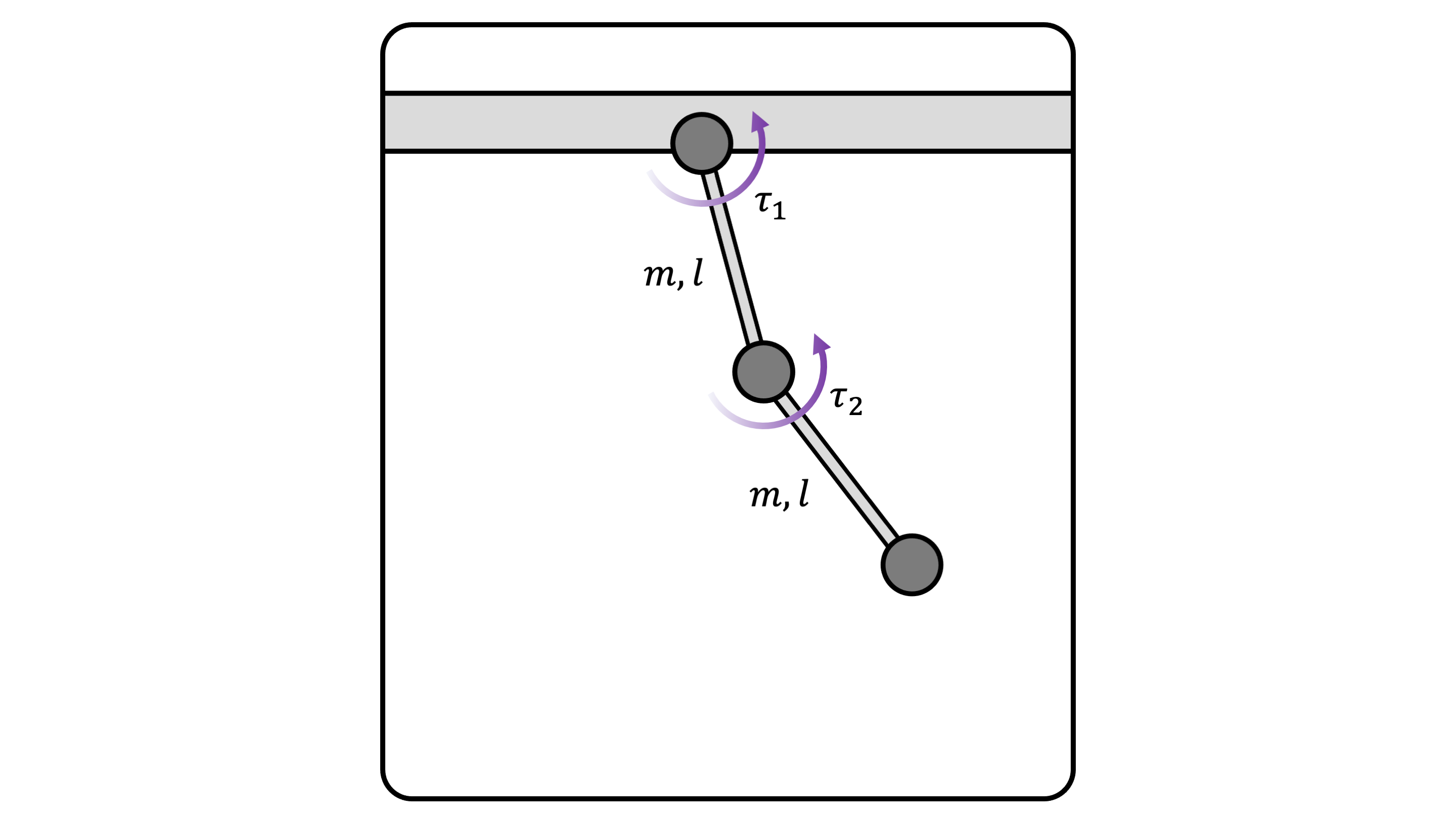
(Figure 1) A double pendulum robot
For the virtual joint trajectory \(\mathbf{q}_0(t)\in\mathbb{R}^2\), we use the minimum-jerk trajectory [8]:
\[ \mathbf{q}_0(t) = \begin{cases} \mathbf{q}_{0,i} & t < t_0 \\ \mathbf{q}_{0,i} + ( \mathbf{q}_{0,f} -\mathbf{q}_{0,i} ) \Big\{ 10 \big( \frac{t-t_0}{D}\big)^3 -15 \big( \frac{t-t_0}{D}\big)^4 +6 \big( \frac{t-t_0}{D}\big)^5 \Big\} & t_0 \le t < t_0 +D \\ \mathbf{q}_{0,f} & t_0+D \le t \\ \end{cases} \] In this equation, \(\mathbf{q}_{0,i}, \mathbf{q}_{0,f} \in\mathbb{R}^2\) are the initial and final (virtual) joint postures, respectively; \(t_0, D \in\mathbb{R}_{>0}\) are the starting time the duration of the movement, respectively.
The results are shown in the video below. For the simulation, we used Explicit-MATLAB. As shown in the videos, it is clear that as the joint stiffness increases, the deviation from the virtual joint posture decreases.