Conservative Force
Moses C. Nah
2023-03-06
Definition
A conservative force is a force that the total mechanical work done in moving a particle between two points is independent of the path taken [1]; [2], [3] As discussed in the previous note, gravitational force is an example of a conservative force.
Properties of Conservative Force
Conservative force has great properties which are worth to be discussed in detail as a separate post.
Property 1: Work Done Along a Closed Trajectory is Zero
Consider two points 1 and 2 in space (Figure 1). Let the work done by a conservative force (vector) field \(\mathbf{F}(\mathbf{r})\) along any path from point 1 to 2 be \(W_{1\rightarrow 2}\) (Figure 1, Left).
Since the total work done by the conservative force \(\mathbf{F}\) is independent of the path take, we can choose any curve connecting from point 1 to 2 and calculate \(W_{1\rightarrow 2}\). Let the curve be \(C_A\) (Figure 1, Right): \[ W_{1\rightarrow 2} = \int_{C_A} \mathbf{F}(\mathbf{r}) \cdot d\mathbf{r} \]
If we simply reverse the curve \(C_A\), we can also calculate the work done by the conservative force field \(\mathbf{F}\) from point 2 to point 1, \(W_{2\rightarrow 1}\), which is simply the negative of \(W_{1\rightarrow 2}\): \[ W_{2\rightarrow 1} = \int_{-C_A} \mathbf{F}(\mathbf{r}) \cdot d\mathbf{r} = -\int_{C_A} \mathbf{F}(\mathbf{r}) \cdot d\mathbf{r} = -W_{1\rightarrow2} \]
By definition, the work done by force \(\mathbf{F}\) is independent of the path taken. Hence, with the curve fixed at point 1 and 2, we can freely deform the curve without changing the value of \(W_{2\rightarrow 1}\). Let the new curve after deformation be \(C_B\) (Figure 1, Right): \[ W_{2\rightarrow 1} = \int_{-C_A} \mathbf{F}(\mathbf{r}) \cdot d\mathbf{r} = \int_{C_B}\mathbf{F}(\mathbf{r}) \cdot d\mathbf{r} \] If we concatenate two curves \(C_A\) and \(C_B\) and make a closed-loop curve \(C\), the work done by the conservative force \(\mathbf{F}\) along that closed-loop curve is zero: \[ W = \oint_C \mathbf{F}(\mathbf{r})\cdot d\mathbf{r} = \int_{C_A} \mathbf{F}(\mathbf{r})\cdot d\mathbf{r} + \int_{C_B}\mathbf{F}(\mathbf{r})\cdot d\mathbf{r} = \int_{C_A} \mathbf{F}(\mathbf{r})\cdot d\mathbf{r} + \int_{-C_A}\mathbf{F}(\mathbf{r})\cdot d\mathbf{r} = 0 \]
Hence, we derive that the work done by the conservative force along any closed curve \(C\) is zero: \[ \oint_C \mathbf{F}(\mathbf{r}) \cdot d\mathbf{r} = 0 \tag{1} \]

(Figure 1) (Left) Possible paths from point 1 to 2. (Right) Under a conservative force field, the work done along the closed path is always zero. Although not depicted on the image, imagine a force field \(\mathbf{F}\) superimposed on the image, i.e., for every point in the image, there is a force vector.
Property 2: Curl of a Conservative Force Field is Zero
Using the Stokes’ Theorem in Equation 1: \[ \oint_C \mathbf{F}(\mathbf{r}) \cdot d\mathbf{r} = \iint_{S} \big\{ \nabla \times \mathbf{F}(\mathbf{r}) \big\} \cdot d \mathbf{S} \tag{2} \] In this equation, \(\nabla \times \mathbf{F}(\mathbf{r})\) is the curl of a force field \(\mathbf{F}(\mathbf{r})\). Recall that the curl operator, \(\nabla \times\), takes a vector (field) as an input and outputs a vector (field). Hence, we can take the dot product with \(d\mathbf{S}\) (Figure 2).
If \(\mathbf{F}\) is a conservative force field, using Property 1 (or Equation 1): \[ \oint_C \mathbf{F}(\mathbf{r}) \cdot d\mathbf{r} = 0 = \iint_{S} \big\{ \nabla \times \mathbf{F}(\mathbf{r}) \big\} \cdot d \mathbf{S} \tag{3} \] To satisfy Equation 3 for any arbitrary closed-loop curve \(C\) and its surface \(S\), it is clear that:1 \[ \nabla \times \mathbf{F}(\mathbf{r}) = \mathbf{0} \tag{4} \] This implies that the curl of a conservative force field is always zero.2
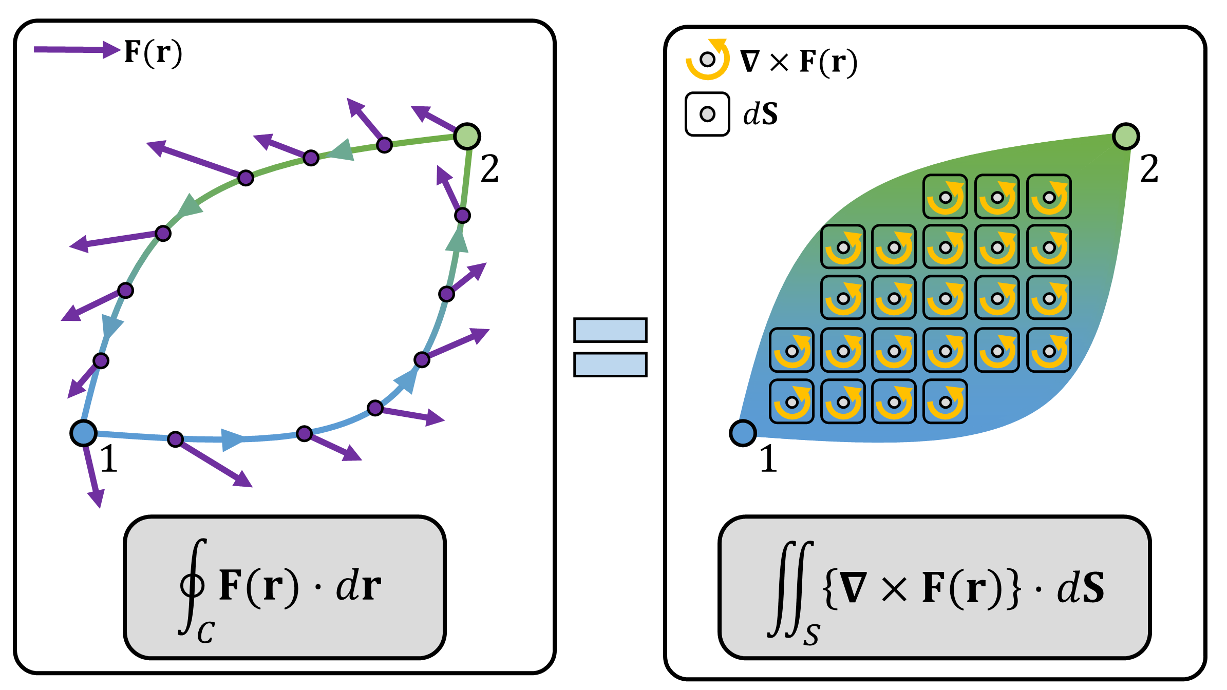
(Figure 2) (Left) The force integration along a closed-loop curve \(C\) (Right) The curl of the force field \(\nabla \times \mathbf{F}\), described as a vector which is going out of the plane, and the infinitesimal surface \(d\mathbf{S}\) with direction along its normal vector. The dot product of \(\nabla \times \mathbf{F}\) and \(d\mathbf{S}\) is taken at each point and integrated along an infinitesimal surface \(d\mathbf{S}\) at that point. Loosely speaking about the intuition of Stokes’ Theorem, the integration of the small rotational flow over the 2D surface is equivalent to the integration of the flow along the 1D line which is the boundary of that surface/
Property 3: Conservative Force Field is the Negative Gradient of a Potential Function
Equation 4 implies that the conservative force field \(\mathbf{F}(\mathbf{r})\) can be described as a gradient of a potential field \(\Phi(\mathbf{r})\). While the detailed proof for this can be derived from Equation 1 with the Fundamental theorem of calculus, we show another perspective using the famous identity: \[ \nabla \times \{ \nabla \Phi(\mathbf{r}) \} = \mathbf{0} \tag{5} \]
Meaning, the curl of the gradient of any scalar field \(\Phi(\mathbf{r})\) is zero.3 Hence, the conservative force field can be written as a gradient of a potential field \(\Phi(\mathbf{r})\): \[ \mathbf{F}(\mathbf{r}) = - \nabla \Phi (\mathbf{r}) \tag{6} \] where the minus sign is simply a matter of convention.
This result is actually quite astonishing. As discussed by Cornelius Lanczos [4]: a single scalar function called a potential function can calculate force, which is a vector that needs more than 1 components to fully describe the components.
Summary
Summarizing, the three main properties of conservative force are:
- The work done by the conservative force along any closed path is zero (Equation 1).
- The curl of a conservative force field is zero (Equation 4).
- The conservative force field can be described as a gradient of a scalar function, which is called the potential function (Equation 6).
Examples
We introduce two simple examples to emphasize the properties of conservative force fields. For that, we discuss about gravitational force field.
Example 1: Gravity, near the Earth’s Surface
Consider a point particle with mass \(m\). Assuming that the particle is sufficiently near the surface of the Earth, for all points, the gravitational force field of the object with mass \(m\) is (Figure 3): \[ \mathbf{F}(\mathbf{r}) = -mg \mathrm{\hat{e}_Y} \tag{7} \]
Based on property 1, the work done by this force field along any closed path is zero. We show this by a simple example shown in Figure 3, Right: \[ \begin{align} W_{A\rightarrow B} &= \int_{3}^{1}-mg \mathrm{\hat{e}_Y} \cdot dy \mathrm{\hat{e}_Y} = -mg \int_{3}^{1}dy = 2mg\\ W_{B\rightarrow C} &= \int_{1}^{3}-mg \mathrm{\hat{e}_Y} \cdot dx \mathrm{\hat{e}_X} = 0 \\ W_{C\rightarrow D} &= \int_{1}^{3}-mg \mathrm{\hat{e}_Y} \cdot dy \mathrm{\hat{e}_Y} = -mg \int_{1}^{3} dy = -2mg \\ W_{D\rightarrow A} &= \int_{3}^{1}-mg \mathrm{\hat{e}_Y} \cdot dx \mathrm{\hat{e}_X} = 0 \\ \\ W &= W_{A\rightarrow B} + W_{B\rightarrow C} + W_{C\rightarrow D} + W_{D\rightarrow A} = 0 \end{align} \] Note that \(W_{B\rightarrow C}\) and \(W_{D\rightarrow A}\) are 0 since \(\mathrm{\hat{e}_X}\) and \(\mathrm{\hat{e}_Y}\) are orthogonal.
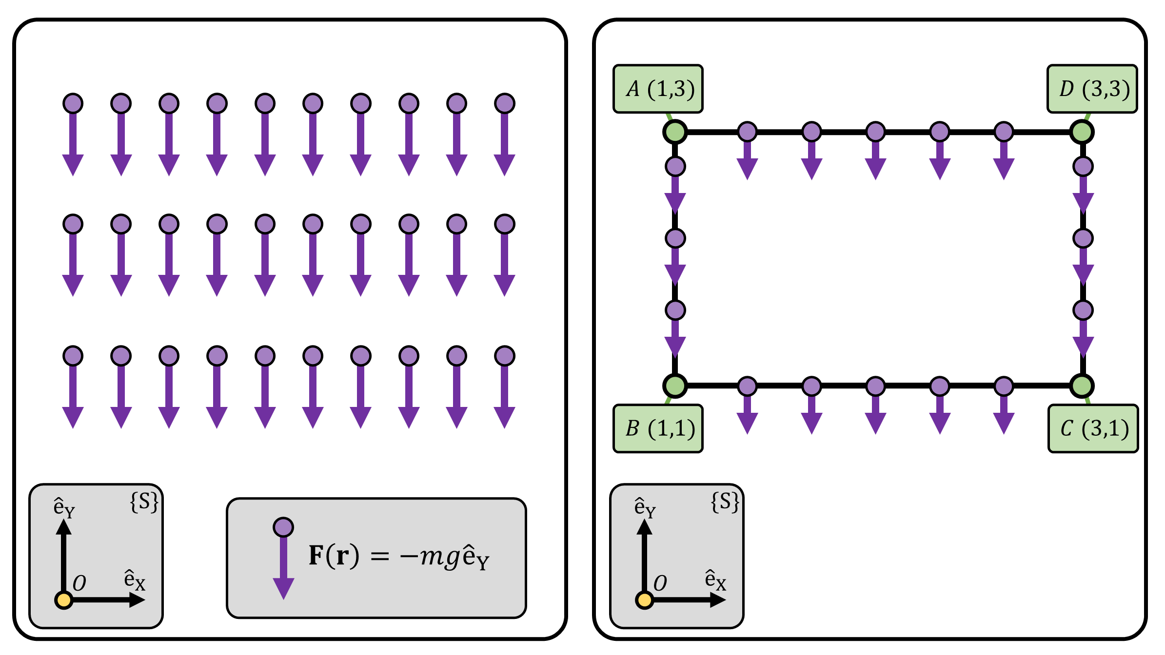
(Figure 3) (Left) Gravitational force field near the Earth’s surface. For all points, the gravitational forces are pointed towards the same direction with same magnitude. (Right) A closed-loop trajectory, \(A\rightarrow B\rightarrow C\rightarrow D\). Given the coordinate frame, the coordinates of points A,B,C,D are (1,1), (3,1), (3,3), (1,3), respectively.
The result from this simple example can be generalized to arbitrary closed-loop path (Figure 4). An infinitesimal part of the curve can be decomposed into parts along \(\mathrm{\hat{e}_X}\) and \(\mathrm{\hat{e}_Y}\). The work done along the \(\mathrm{\hat{e}_X}\) parts is always zero, and collecting the remaining \(\mathrm{\hat{e}_Y}\) parts and summing them up also results to zero, since it is a closed-loop trajectory.
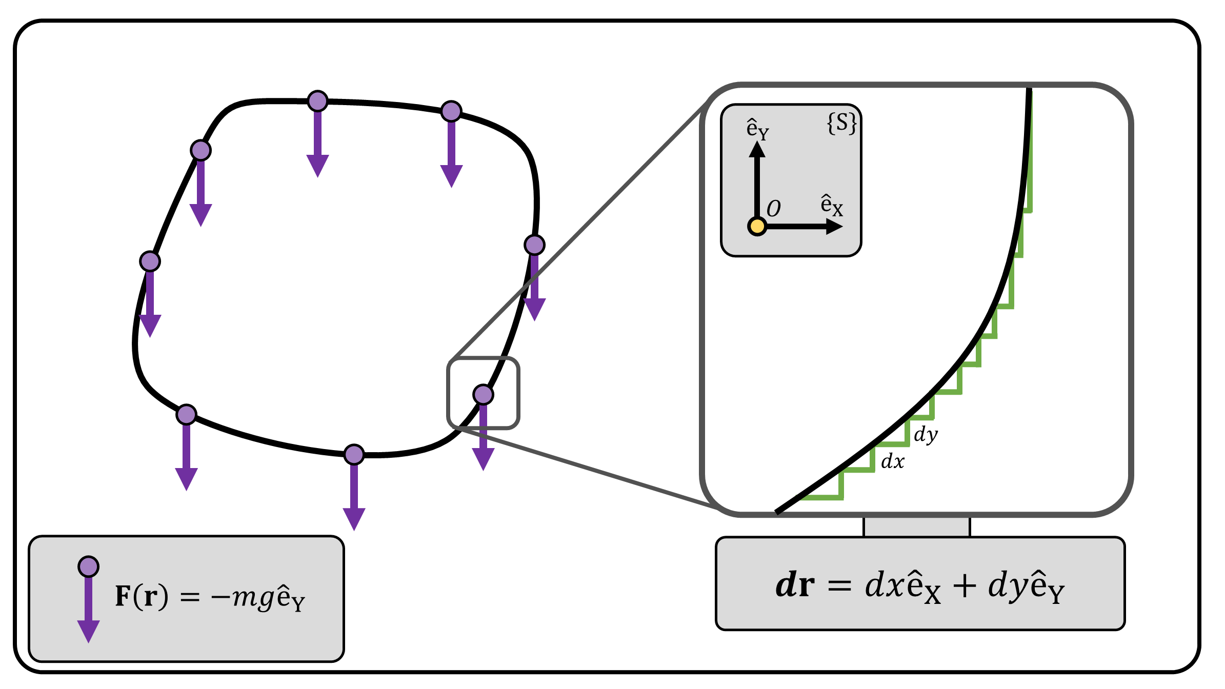
(Figure 4) An arbitrary closed-loop trajectory. We can simply collect all the \(dx\) and \(dy\) parts and reshape it as a rectangle, which leads us back to the example shown in Figure 3.
Example 2: Gravity, Outer Space
Consider a particle with mass \(m\) that is outer space and under the influence of gravity of the Earth. The Newton’s law of universal gravitation shows that the force experienced by mass \(m\) is: \[ \mathbf{F}(\mathbf{r}) = -G\frac{mM}{r^2} \mathrm{\hat{e}_r } \] In this equation, \(G\) is the gravitational constant; \(M\) is the mass of the Earth; \(r\) is the distance measured from the Earth center to mass \(m\); \(\mathrm{\hat{e}_r}\) is the basis vector of the Polar coordinate system.4
For Polar coordinate system: \[ d\mathbf{r} = dr\mathrm{\hat{e}_r} +r d\theta \mathrm{\hat{e}_\theta } \]
Again, gravitational force field is a conservative force. Hence, the work done by the force along a closed trajectory is zero. For the example shown in Figure 5, the work done along path \(B \rightarrow C\), \(D \rightarrow E\), and \(F\rightarrow A\) are zero since the force is orthogonal to the path taken. Hence, we only consider path \(A\rightarrow B\), \(C\rightarrow D\), and \(E\rightarrow F\): \[ \begin{align} W_{A\rightarrow B} &= \int_{r_1}^{r_3}-G\frac{mM}{r^2}\mathrm{\hat{e}_r} \cdot d\mathbf{r} = \int_{r_1}^{r_3}-G\frac{mM}{r^2}dr = GmM\Big[ \frac{1}{r_3} - \frac{1}{r_1} \Big] \\ W_{C\rightarrow D} &= \int_{r_3}^{r_4}-G\frac{mM}{r^2}\mathrm{\hat{e}_r} \cdot d\mathbf{r} = \int_{r_3}^{r_4}-G\frac{mM}{r^2}dr = GmM\Big[ \frac{1}{r_4} - \frac{1}{r_3} \Big] \\ W_{E\rightarrow F} &= \int_{r_4}^{r_1}-G\frac{mM}{r^2}\mathrm{\hat{e}_r} \cdot d\mathbf{r} = \int_{r_4}^{r_1}-G\frac{mM}{r^2}dr = GmM\Big[ \frac{1}{r_1} - \frac{1}{r_4} \Big] \\ \\ W &= W_{A\rightarrow B} + W_{B\rightarrow C} + W_{C\rightarrow D} + W_{D\rightarrow E} + W_{E\rightarrow F} + W_{F\rightarrow A} = 0 \end{align} \]
And using the same logic shown in Figure 4, this can be generalized to any arbitrary closed-loop trajectory. Given an arbitrary closed-loop trajectory, the trajectory can be approximated by a series of radial and circumferential steps. The work done along the circumferential steps can be neglected since the displacement and force are orthogonal. Hence, the radial steps are only accounted for the calculation, and eventually the work done along the closed-loop trajectory is zero [5].
Note that Under the choice of Polar coordinate system, the potential field \(\Phi(\mathbf{r})\) is simply: \[ \Phi(r,\theta) = G\frac{mM}{r} \]
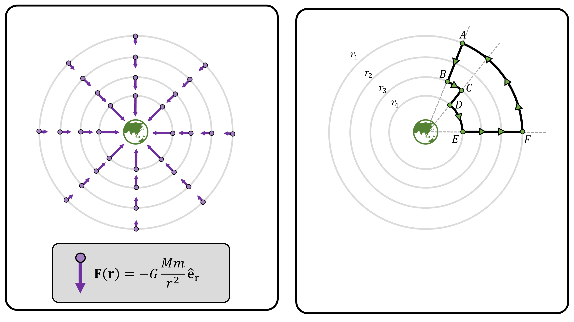
(Figure 5) (Left) Gravitational force field around the Earth. The magnitude (or the length) of the force gets smaller, inversely proportional to the square of the distance. (Right) An exemplary closed-loop trajectory. Grey lines depict the concentric circles radiating out from the origin (i.e., Earth) of the polar coordinate system.
References
In case if you are not convinced about Equation 4, think about an infinitesimal-sized closed-loop curve at each point. Even that curve must satisfy Equation 3, which leads us to Equation 4 ↩︎
Be careful! \(\mathbf{0}\) is not a zero scalar. It is a zero vector↩︎
For people who are familiar with tensor notations, Equation 5 can be proved with few lines. The \(i\)-th component of \(\nabla \times ( \nabla \Phi )\) can be written as: \[ \big\{\nabla \times ( \nabla \Phi(\mathbf{r}) )\big\}_i = \epsilon_{ijk} \partial_j (\partial_k\Phi(\mathbf{r}) ) \] In this equation, \(\epsilon\) denotes the Levi-Civita symbol, and \(\partial_j\) is the partial derivative with respect to the \(j\)-th component. If we switch index \(j\) and \(k\): \[ \begin{align} \big\{\nabla \times ( \nabla \Phi(\mathbf{r}) )\big\}_i &= \epsilon_{ikj} \partial_k (\partial_j\Phi(\mathbf{r})) = -\epsilon_{ijk} \partial_k (\partial_j\Phi(\mathbf{r}) ) = -\epsilon_{ijk} \partial_j (\partial_k\Phi(\mathbf{r}) ) = -\big\{\nabla \times ( \nabla \Phi(\mathbf{r}) )\big\}_i \\ \big\{\nabla \times ( \nabla \Phi(\mathbf{r}) )\big\}_i &= 0 \end{align} \] The minus sign of the second equality uses the antisymmetric property of Levi-Civita symbol. The third equality uses the Schwarz’s Thereom — the commutativity of partial derivatives. Kudos to Prof. Balakrishnan, one of my favorite professors, who have explained this formula here. ↩︎
One can check that \(g=9.81=GM/R^2\), where \(R\) is the radius of the Earth.↩︎