Adaptive Control
Moses C. Nah
2023-03-17
Introduction
Consider the manipulator equation of an open-chain \(n\)-DOF robot [1], [2]:
\[ \mathbf{M(q)\ddot{q}+C(q,\dot{q})\dot{q}+g(q)}=\boldsymbol{\tau}_{in} \tag{1} \] We assume no external forces applied to the robot.
Several robotic control approaches assume the knowledge of the exact values of the mass matrix \(\mathbf{M(q)}\), Coriolis/centrifugal Matrix \(\mathbf{C(q,\dot{q})}\), and gravity (co-)vector \(\mathbf{g(q)}\). However in practice, this is often not the case. The presence of uncertainty on the inertial properties of the robot complicates the control problem.
In this post, we introduce Adaptive Control of robot manipulators, introduced by Slotine and Li [3]. Adaptive control achieves tracking control under the uncertainty (or without the exact knowledge) of the inertial parameters.
The Unknown Inertial Parameters
In detail, for each rigid body of the \(n\)-DOF robot manipulator, there are 10 unknown inertial parameters:
- The mass of the \(i\)-th link, \(m_i\) (1 parameter)
- The first mass moment (i.e., mass times the location of the Center of Mass) of the \(i\)-th link \(m_i\mathbf{c}_i=(mc_{i,x}, mc_{i,y}, mc_{c,z})\), represented in body-fixed coordinate (3 parameters)
- The inertia matrix about the body-fixed coordinate, \(I_{i,xx}, I_{i,xy}, I_{i,xz}, I_{i,yy}, I_{i,yz}, I_{izz}\) (6 parameters)
The 10 unknown inertial parameters of the \(i\)-th link can be composed as a single array \(\mathbf{a}_i\in\mathbb{R}^{10}\): \[ \mathbf{a}_i = (m_i, ~ mc_{x,i}, ~mc_{y,i}, ~mc_{z,i}, ~I_{xx,i}, ~I_{xy,i}, ~I_{xz,i}, ~I_{yy,i}, ~I_{yz,i}, ~I_{zz,i} ) \] Therefore, the unknown inertial parameters of the \(n\)-DOF robot manipulator can be collected as a single constant array \(\mathbf{a}:=(\mathbf{a}_1, \mathbf{a_2}, \cdots, \mathbf{a}_n)\in\mathbb{R}^{10n}\). Adaptive control achieves tracking control under the uncertainty of \(\mathbf{a}\).
Adaptive Control
Adaptive control consists of a (1) feedback controller and an (2) adaptation law.
Feedback Controller
The control objective is to track a desired joint trajectory \(\mathbf{q}_d(t)\), under the uncertainty of \(\mathbf{a}\).
It is commonly known that the left-hand side of Equation 1 can be represented linearly in system inertial parameters \(\mathbf{a}\) [3], [4]: \[ \mathbf{M(q)\ddot{q}+C(q,\dot{q})\dot{q}+g(q)=\mathbf{Y}(q,\dot{q},\ddot{q}})\mathbf{a} \]
Adaptive control uses the following feedback controller: \[ \boldsymbol{\tau}_{in}=\mathbf{\hat{M}(q)\ddot{q}_r+\hat{C}(q,\dot{q})\dot{q}_r+\hat{g}(q)-K_Ds} = \mathbf{Y}(\mathbf{\ddot{q}_r}, \mathbf{\dot{q}_r}, \mathbf{\dot{q}}, \mathbf{q})\hat{\mathbf{a}}-\mathbf{K_Ds} \tag{2} \] In these equations, \(\mathbf{\ddot{q}_r}, \mathbf{\dot{q}_r}\in\mathbb{R}^n\) are reference joint acceleration and joint velocity, respectively; \(\mathbf{s}\in\mathbb{R}^{n}\) is the sliding variable; \(\mathbf{K}_D\in\mathbb{R}^{n\times n}\) is a constant symmetric positive definite matrix; \(\hat{\mathbf{a}}\in\mathbb{R}^{10n}\) is the estimation of the unknown inertial parameters which is randomly initialized: \[ \mathbf{s}=\mathbf{\dot{\tilde{q}}}+\boldsymbol{\Lambda}\mathbf{\tilde{q}}, ~~~~~~~~~~ \mathbf{\dot{q}_r}= \mathbf{\dot{q}_d}+\boldsymbol{\Lambda}(\mathbf{q_d-q}), ~~~~~~~~~~ \mathbf{s}=\mathbf{\dot{q}-\dot{q}_r}, ~~~~~~~~~~ \mathbf{\tilde{q}=q-q_d} \] In these equations, \(\boldsymbol{\Lambda}\in\mathbb{R}^{n\times n}\) is a constant symmetric positive definite matrix.
By applying \(\boldsymbol{\tau}_{in}\), the closed-loop dynamics results in the following differential equation: \[ \begin{align*} \mathbf{M(q)\underbrace{(\ddot{q}-\ddot{q}_r)}_{=\dot{\mathbf{s}}}+C(q,\dot{q})\underbrace{(\dot{q}-\dot{q}_r)}_{=\mathbf{s}}} &=\{\mathbf{\hat{M}(q)-M(q))\ddot{q}_r + \{\hat{C}(q,\dot{q})-C(q,\dot{q})\}\dot{q}_r+\{\hat{g}(q)-g(q)\}-K_Ds} \\ \mathbf{M(q)\dot{s}+\{C(q,\dot{q})+K_D\}s}&=\mathbf{Y(q,\dot{q},\dot{q}_r, \ddot{q}_r)\{\hat{\mathbf{a}}-\mathbf{a}\}} := \mathbf{Y(q,\dot{q},\dot{q}_r, \ddot{q}_r)\tilde{a}} \end{align*} \] In these equation, \(\mathbf{\tilde{a}}:=\mathbf{\hat{a}-a}\in\mathbb{R}^{10n}\) is the error of the estimated and the actual inertial parameters.
Adaptation Law and its Stability Analysis
We define scalar function \(V(\mathbf{s},\mathbf{\tilde{a}})\): \[ V(\mathbf{s},\mathbf{\tilde{a}}) := \frac{1}{2}\mathbf{s^{T}M(q)s} + \frac{1}{2}\mathbf{\tilde{a}^T}\boldsymbol{\Gamma^{-1}}\mathbf{\tilde{a}} \] In this equation, \(\boldsymbol{\Gamma}\in\mathbb{R}^{10n\times 10n}\) is a constant symmetric positive definite matrix.
The time derivative of \(V(\mathbf{s},\mathbf{\tilde{a}})\): \[ \begin{align*} \frac{d}{dt}V(\mathbf{s},\mathbf{\tilde{a}}) &= \mathbf{s^{T}M(q)\dot{s}} + \frac{1}{2}\mathbf{s^{T}\dot{M}(q)s} + \mathbf{\tilde{a}^T}\boldsymbol{\Gamma^{-1}}\mathbf{\dot{\hat{a}}} \\ &= \mathbf{s^T}\big\{\mathbf{Y(q,\dot{q},\dot{q}_r, \ddot{q}_r)\tilde{a}} - \mathbf{C(q,\dot{q})s -K_Ds} \big\} + \frac{1}{2}\mathbf{s^{T}\dot{M}(q)s}+ \mathbf{\tilde{a}^T}\boldsymbol{\Gamma^{-1}}\mathbf{\dot{\hat{a}}} \\ &= \underbrace{\mathbf{s^T}\Big\{ \frac{1}{2}\mathbf{\dot{M}(q)-C(q,\dot{q})}\Big\}\mathbf{s}}_{=0} + \mathbf{s^T}\mathbf{Y(q,\dot{q},\dot{q}_r, \ddot{q}_r)\tilde{a}}+ \mathbf{\tilde{a}^T}\boldsymbol{\Gamma^{-1}}\mathbf{\dot{\hat{a}}} - \mathbf{s^TK_Ds} \\ &= \mathbf{s^T}\mathbf{Y(q,\dot{q},\dot{q}_r, \ddot{q}_r)\tilde{a}}+ \mathbf{\tilde{a}^T}\boldsymbol{\Gamma^{-1}}\mathbf{\dot{\hat{a}}} - \mathbf{s^TK_Ds} \end{align*} \] Recall that \(\mathbf{a}\) is constant, hence \(\mathbf{a}\) vanishes under time derivative. Moreover, for the third line of the equation, we use the well-known property [3]: \[ \forall \mathbf{v}\in\mathbb{R}^{n}:~~ \mathbf{v^{T}}\Big\{ \frac{1}{2}\dot{\mathbf{M}}(\mathbf{q})-\mathbf{C(q,\dot{q})}\Big\}\mathbf{v} = 0 \] Here, the key idea of adaptive control emerges. If we define the adaptation law (or update rule) for \(\mathbf{\hat{a}}\) as: \[ \mathbf{\dot{\hat{a}}}:=-\boldsymbol{\Gamma}\mathbf{Y^T(q,\dot{q},\dot{q}_r, \ddot{q}_r)}\mathbf{s} \tag{3} \] The time derivative of \(V(\mathbf{s},\mathbf{\tilde{a}})\) is negative semi-definite: \[ \frac{d}{dt}V(\mathbf{s},\mathbf{\tilde{a}}) = - \mathbf{s^TK_Ds} \le 0 \] Finally, under the adaptation law of Equation 3, the double time derivative of \(V(\mathbf{s},\mathbf{\tilde{a}})\) is also bounded: \[ \begin{align*} \forall t>0: \exists \alpha>0: \Bigg| \frac{d^2}{dt^2}V(\mathbf{s},\mathbf{\tilde{a}})\Bigg| &= \Big| 2\mathbf{s^TK_D\dot{s}} \Big| \\ &= \bigg| -2\mathbf{s^TK_D}\big\{ \mathbf{M(q)}^{-1} ~ ( \mathbf{Y(q,\dot{q},\dot{q}_r, \ddot{q}_r)\tilde{a} - C(q,\dot{q})s-K_Ds } )~ \big\} \bigg| \le \alpha \end{align*} \] Summarizing, under the adaptation law of Equation 3, scalar function \(V(\mathbf{s},\mathbf{\tilde{a}})\) satisfies the three conditions of Barbalat’s Lemma:1 \[ \begin{align*} (1)~~ V(\mathbf{s},\mathbf{\tilde{a}}) &\ge 0 \\ (2)~~ \dot{V}(\mathbf{s},\mathbf{\tilde{a}}) &\le0 \\ (3)~~ \ddot{V}(\mathbf{s},\mathbf{\tilde{a}}) &~\text{is Bounded} \end{align*} ~~~ \Longrightarrow ~~~ \dot{V}(\mathbf{s},\mathbf{\tilde{a}}) \rightarrow 0 ~~ \text{as} ~~ t\rightarrow \infty \] Since \(\mathbf{K_D}\) is positive definite, \(\mathbf{s}\rightarrow 0\), i.e., tracking control is achieved \(\mathbf{q}(t)\rightarrow \mathbf{q}_d(t)\).
Summary
The adaptive control is achieved by a feedback controller and the corresponding adaptation law: \[ (1) ~~\boldsymbol{\tau}_{in}= \mathbf{Y}(\mathbf{\ddot{q}_r}, \mathbf{\dot{q}_r}, \mathbf{\dot{q}}, \mathbf{q})\hat{\mathbf{a}}-\mathbf{K_Ds} ~~~~~~ (2)~~\mathbf{\dot{\hat{a}}}:=-\boldsymbol{\Gamma}\mathbf{Y^T(q,\dot{q},\dot{q}_r, \ddot{q}_r)}\mathbf{s} \]
The choice of gains, refer to [5]
Example — Double Pendulum
Consider a 2-DOF double pendulum robot, which consists of two links with mass \(m_1\), \(m_2\), and length \(l_1\), \(l_2\) (known). The center of mass location of the two links are \(c_{1,x}:=l_{c1}\) and \(c_{2,x}:=l_{c2}\), along \(\mathrm{\hat{e}}_{x,1}\) and \(\mathrm{\hat{e}}_{x,2}\) of frame \(\{1\}\) and \(\{2\}\), respectively. The moment of inertia of two links about \(\mathrm{\hat{e}}_{z,1}\) and \(\mathrm{\hat{e}}_{z,2}\) (i.e., about the pivots) are \(I_{1,zz}:=I_1\), \(I_{2,zz}:=I_2\), respectively (Figure 1).
The equation of motion of the system is well-known [6]: \[ \begin{align*} \underbrace{ \begin{pmatrix} \tau_1 \\ \tau_2 \end{pmatrix}}_{=\boldsymbol{\tau}_{in}} &= \underbrace{ \begin{pmatrix} I_1+I_2 + m_2l_1^2+2m_2l_1l_{c2}\cos q_2 & I_2 + m_2l_1l_{c2}\cos q_2 \\ I_2 + m_2l_1l_{c2}\cos q_2 & I_2 \end{pmatrix} }_{=\mathbf{M(q)}} \begin{pmatrix} \ddot{q}_1 \\ \ddot{q}_2 \end{pmatrix} \\ &+ \underbrace{ \begin{pmatrix} -2m_2l_1l_{c2}\dot{q}_2\sin q_2 & -m_2l_1l_{c2}\dot{q}_2\sin q_2 \\ \phantom{-2}m_2l_1l_{c2}\dot{q}_1\sin q_2 & 0 \end{pmatrix} }_{=\mathbf{C(q,\dot{q})}} \begin{pmatrix} \dot{q}_1 \\ \dot{q}_2 \end{pmatrix} + \underbrace{ \begin{pmatrix} -m_1gl_{c1}\sin q_1 - m_2g\{l_1\sin(q_1) + l_{c2}\sin(q_1+q_2)\} \\ -m_2gl_{c2}\sin(q_1+q_2) \end{pmatrix} }_{=\mathbf{g(q)}} \end{align*} \]
The unknown inertial parameters are \(\mathbf{a}:=( m_1, m_1l_{c1}, I_1, m_2, m_2l_{c2}, I_2)\). The feedback control law is (Equation 2): \[ \boldsymbol{\tau}_{in} = \mathbf{Y}(\mathbf{\ddot{q}_r}, \mathbf{\dot{q}_r}, \mathbf{\dot{q}}, \mathbf{q})\hat{\mathbf{a}}-\mathbf{K_Ds} \] The detailed \(\mathbf{Y}(\mathbf{\ddot{q}_r}, \mathbf{\dot{q}_r}, \mathbf{\dot{q}}, \mathbf{q}) \in \mathbb{R}^{2\times 6}\) matrix is: \[ \mathbf{Y}(\mathbf{\ddot{q}_r}, \mathbf{\dot{q}_r}, \mathbf{\dot{q}}, \mathbf{q}) = \begin{pmatrix} 0 & -g\sin q_1 & \ddot{q}_{r,1} & Y_{14} & Y_{15} & \ddot{q}_{r,1} + \ddot{q}_{r,2} \\ 0 & 0 & 0 & 0 & Y_{25} & \ddot{q}_{r,1} + \ddot{q}_{r,2} \end{pmatrix} \] \[ \begin{align} Y_{14} &= \ddot{q}_{r,1}l_1^2 - gl_1\sin q_1 \\ Y_{15} &= 2\ddot{q}_{r,1}l_1\cos q_2 - g\sin(q_1+q_2) + \ddot{q}_{r,2}l_1 \cos q_2 - 2\dot{q}_2\dot{q}_{r,1}l_1\sin q_2-\dot{q}_2\dot{q}_{r,2}l_1\sin q_2 \\ Y_{25} &= \ddot{q}_{r,1}l_1\cos q_2 - g\sin(q_1+q_2) + \dot{q}_1\dot{q}_{r,1}l_1\sin q_2 \end{align} \] In these equations, \(\mathbf{\ddot{q}_r} := (\ddot{q}_{r,1}, \ddot{q}_{r,2})\), \(\mathbf{\dot{q}_r} := (\dot{q}_{r,1}, \dot{q}_{r,2})\).
One should keep in mind that for deriving the \(\mathbf{Y}(\mathbf{\ddot{q}_r}, \mathbf{\dot{q}_r}, \mathbf{\dot{q}}, \mathbf{q})\) matrix, the arguments of the mass matrix \(\mathbf{M(q)}\), Coriolis/centrifugal matrix \(\mathbf{C(q,\dot{q})}\), are not the reference velocity, but the joint angle \(\mathbf{q}\) and joint velocity \(\mathbf{\dot{q}}\) given from the feedback.
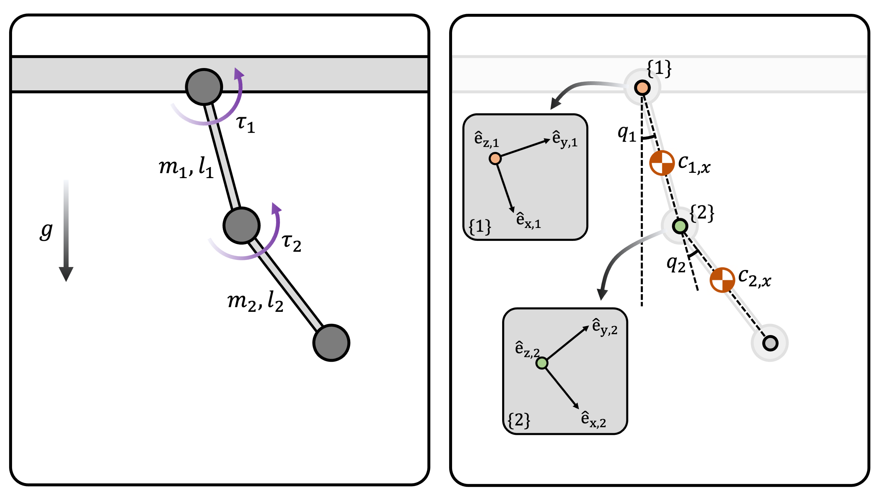
(Figure 1) A double pendulum.
The examples can be checked here (TBD).
Question: Parameter Estimation via Adaptive Control?
(TBD)
References
Note that the sliding variable \(\mathbf{s}=\mathbf{s}(t)\), i.e., a function of time due to \(\mathbf{q}_d(t)\). Hence, the closed-loop dynamics is a non-autonomous system. Therefore, we cannot use La-Salle’s invariant set theorem and instead need to use Barbalat’s Lemma. ↩︎