Lagrange Multiplier Method
Moses C. Nah
2023-02-26
Motivation
Suppose we want to minimize (or optimize) function \(f(x,y)\) where \(f: \mathbb{R} \times \mathbb{R} \longrightarrow \mathbb{R}\) has two variables. However, there is an (equality) constraint \(g(x,y)=c\), where and \(g: \mathbb{R} \times \mathbb{R} \longrightarrow \mathbb{R}\), and \(c\) is a constant. Assume that both, \(f(x,y)\) and \(g(x,y)\) are continuously differentiable for each \(x\) and \(y\).
This is a typical optimization problem with equality constraint:
\[ \begin{align*} \begin{split} \min_{x,y} ~~ &f(x,y) \\ \text{subject to} ~~ &g(x,y)=c \end{split}\tag{1} \end{align*} \] Consider a small displacement (\(\delta x\), \(\delta y\)) around point \((x,y)\). For the point \((x,y)\) to be the local minima (or optima) of function \(f(x,y)\), the change rate of change of function \(f(x,y)\) must be zero for any displacement (\(\delta x\), \(\delta y\)):
\[ \delta f(x,y)= \frac{\partial f}{\partial x} \delta x + \frac{\partial f}{\partial y} \delta y = 0 \tag{2} \] If there exists no constraint for the optimization, the goal is to find points \((x,y)\) which make the partial derivatives \(\partial f/\partial x\) and \(\partial f/\partial y\) zero. Once you find the point, it is well known that analyzing the Hessian matrix of function \(f(x,y)\) at point \((x,y)\) determines whether point \((x,y)\) is a local minimum, local maximum, or a saddle point.
However, due to the equality constraint \(g(x,y)=c\), there exists a constraint on displacement (\(\delta x\), \(\delta y\)): \[ \delta g(x,y)= \frac{\partial g}{\partial x} \delta x + \frac{\partial g}{\partial y} \delta y = 0 \tag{3} \] Equations 2 and 3 can be written as: \[ \renewcommand{\arraystretch}{1.4} \begin{pmatrix} \frac{\partial f}{\partial x} & \frac{\partial f}{\partial y} \\ \frac{\partial g}{\partial x} & \frac{\partial g}{\partial y} \end{pmatrix} \begin{pmatrix} \vphantom{\frac{\partial f}{\partial x}} \delta x \\ \vphantom{\frac{\partial f}{\partial x}} \delta y \end{pmatrix} = \begin{pmatrix} \vphantom{\frac{\partial f}{\partial x}} 0 \\ \vphantom{\frac{\partial f}{\partial x}} 0 \end{pmatrix} \] To have a non-trivial solution for \((\delta x, \delta y)\), the determinant of the matrix must be zero, i.e., the rows (or columns) must be mutually independent. This can be expressed as: \[ \Big( \frac{\partial f}{\partial x}, \frac{\partial f}{\partial y} \Big) + \lambda \Big( \frac{\partial g}{\partial x}, \frac{\partial g}{\partial y} \Big)=\mathbf{0} ~~~~~~~~~~ \nabla f+\lambda \nabla g = \mathbf{0} \tag{4} \] In these equations, \(\lambda\) is a non-negative scalar value; \(\nabla f\) and \(\nabla g\) are the gradient of function \(f(x,y)\) and \(g(x,y)\), respectively. In other words, \(\nabla f\) should be parallel to \(\nabla g\) at the optimal point.
We now show the ingenuity of Lagrange. We define a new function \(L(x,y,\lambda)\): \[ L(x,y,\lambda) := f(x,y) + \lambda (g(x,y)-c) \] To find the optimal point of function \(L(x,y,\lambda)\), we find the point where the gradient of function \(L(x,y,\lambda)\) vanishes to a zero vector: \[ \begin{align*} \frac{\partial L}{\partial x}: & ~~~ \frac{\partial f}{\partial x} + \lambda \frac{\partial g}{\partial x}=0 \\ \frac{\partial L}{\partial y}: & ~~~ \frac{\partial f}{\partial y} + \lambda \frac{\partial g}{\partial y}=0 \\ \frac{\partial L}{\partial \lambda}: & ~~~ g(x,y)-c=0 \end{align*} \] Remarkably, the first two conditions correspond to Equation 4, and the third condition is the given equality constraint of Equation 1. This is the Lagrange multiplier method, which changes a constrained optimization problem to an unconstrained optimization, by introducing Lagrange multiplier \(\lambda\). Loosely speaking, the Lagrange method loosen up the equality constraint by expanding the variables of the function.
Derivation (Advanced)
We introduce a wonderful derivation of Lagrange multiplier method introduced by Lanczos [1]. Consider a typical multivariate optimization problem: \[ \begin{align*} \begin{split} \min_{x_1,x_2,\cdots x_n} ~~ &f(x_1,x_2,\cdots,x_n) \\ \text{subject to} ~~ &g(x_1,x_2,\cdots,x_n)=c \end{split} \end{align*} \] As shown in Equation 2 and 3, at the optimal point the variation of both, \(f(x_1,x_2,\cdots, x_n)\) and \(g(x_1,x_2,\cdots, x_n)\) must vanish: \[ \begin{align*} & \frac{\partial f}{\partial x_1} \delta x_1 + \frac{\partial f}{\partial x_2} \delta x_2 + \cdots + \frac{\partial f}{\partial x_n} \delta x_n = 0 \tag{5} \\ & \frac{\partial g}{\partial x_1} \delta x_1 + \frac{\partial g}{\partial x_2} \delta x_2 + \cdots + \frac{\partial g}{\partial x_n} \delta x_n = 0 \tag{6}\\ \end{align*} \] Due to Equation 6, variation \(\delta x_1, \delta x_2, \cdots, \delta x_n\) are linearly dependent. Hence, without the loss of generality, variation \(\delta x_n\) with a non-zero coefficient can be substituted at Equation 5, and the optimization of \(n\) variables is reduced to an optimization of \(n-1\) variables. The problem reduces to finding the point which vanishes the coefficients \(\delta x_1, \delta x_2, \cdots, \delta x_n\).
While this method is correct, a better method exists. Since both Equations 5 and 6 are zero, it is obviously permissible to multiply a undetermined factor \(\lambda\) on one of the equations and merge the two: \[ \begin{align*} \frac{\partial f}{\partial x_1} \delta x_1 + \frac{\partial f}{\partial x_2} \delta x_2 + \cdots + \frac{\partial f}{\partial x_n} \delta x_n + \lambda\bigg( \frac{\partial g}{\partial x_1} \delta x_1 + \frac{\partial g}{\partial x_2} \delta x_2 + \cdots + \frac{\partial g}{\partial x_n} \delta x_n \bigg) &= 0 \\ \bigg( \frac{\partial f}{\partial x_1} + \lambda\frac{\partial g}{\partial x_1} \bigg)\delta x_1 + \bigg( \frac{\partial f}{\partial x_2} + \lambda\frac{\partial g}{\partial x_2} \bigg)\delta x_2 + \cdots + \bigg( \frac{\partial f}{\partial x_n} + \lambda\frac{\partial g}{\partial x_n} \bigg)\delta x_n &= 0 \end{align*} \] While the total sum of \(n\) terms is zero, each value of the sum is not zero. As our goal is to eliminate \(\delta x_n\), we can choose \(\lambda\) that eliminates the coefficient of \(\delta x_n\): \[ \frac{\partial f}{\partial x_n} + \lambda \frac{\partial g}{\partial x_n} = 0 \tag{7} \] Once we choose \(\lambda\) that eliminates the \(\delta x_n\) term in the sum, the summation of \(n\) terms reduces to the summation of \(n-1\) terms: \[ \sum_{i=1}^{n-1}\bigg( \frac{\partial f}{\partial x_i} + \lambda\frac{\partial g}{\partial x_i} \bigg) \delta x_i = 0 \tag{8} \] Since we eliminate \(\delta x_n\) via \(\lambda\), Equation 8 should be satisfied for any arbitrary variation of \(\delta x_1, \delta x_2, \cdots \delta x_{n-1}\). This implies that the coefficients of \(\delta x_1, \delta x_2, \cdots \delta x_{n-1}\) must be zero. Summarizing this result with Equation 7, we have: \[ \forall i\in\{1,2,\cdots n\}: ~~ \frac{\partial f}{\partial x_i} + \lambda \frac{\partial g}{\partial x_i} = 0 \tag{9} \] Direct quote from Lanczos [1], we now express the result of our deduction in a much striking form. Equation 9 and the equality constraint can be solve by optimizing an unconstrained optimization problem of the function \(L(x_1, x_2, \cdots, x_n, \lambda)\): \[ \begin{align} L(x_1, x_2, \cdots, x_n, \lambda) &= f(x_1,x_2,\cdots,x_n) + \lambda g(x_1, x_2 \cdots, x_n) \\ \\ \frac{\partial L}{\partial x_1}&: ~~~ \frac{\partial f}{\partial x_1} + \lambda \frac{\partial g}{\partial x_1} = 0\\ & ~~~~~~~~~~~~ \vdots \\ \frac{\partial L}{\partial x_n}&: ~~~ \frac{\partial f}{\partial x_n} + \lambda \frac{\partial g}{\partial x_n} = 0\\ \frac{\partial L}{\partial \lambda} &:~~~ g(x_1,x_2,\cdots,x_n) -c = 0 \end{align} \] Hence, the Lagrange Multiplier Method
Generalization to \(m\) equality constraints is immediate. Let \(\mathbf{x}:=(x_1,x_2,\cdots,x_n)\) and \(\boldsymbol{\lambda}:=(\lambda_1, \lambda_2, \cdots, \lambda_m)\). Given \(m\) equality constraints of \(g_i(\mathbf{x})=c_i\) for \(i\in\{1,2,\cdots. m\}\), the constrained optimization problem reduces to an unconstrained optimization problem of function \(L(\mathbf{x},\boldsymbol{\lambda})\): \[ L(\mathbf{x},\boldsymbol{\lambda}) = f(\mathbf{x}) + \sum_{i=1}^{m}\lambda_i (g_i(\mathbf{x})-c_i) \]
An Example
Consider the following optimization problem: \[ \begin{align*} \begin{split} \min_{x,y} ~~ & x+y \\ \text{subject to} ~~ & x^2+y^2=1 \end{split} \end{align*} \]
Method 1
Without using the Lagrange Multiplier method, we simply take the variation of the equality constraint: \[ x^2 + y^2 = 1 ~~~~~~~~~~ 2x \delta x + 2y \delta y = 0 ~~~~~~~~~~ \delta x = -\frac{y}{x}\delta y ~~~~ \text{for} ~~~~ x\neq0 \] Note that for \(x=0\), then \(\delta y\) is zero, which makes sense (Figure 1). The function to minimize is \(f(x,y)=x+y\). The variation of function \(f(x,y)\) is: \[ \delta f = 1\delta x + 1\delta y = \Big(-\frac{y}{x}+1\Big)\delta x ~~~~~~~ x^* = y^* \] To have an optimal value, the coefficient of \(\delta x\) should be zero. This implies that \(x\) and \(y\) coordinates of the optimal point \(x^*\), \(y^*\) is equal. Using the equality constraint, we have \(x^*=y^*=\pm\frac{1}{\sqrt{2}}\). Thus we have the minimum point \((x^*, y^*)=\big(-\frac{1}{\sqrt{2}}, -\frac{1}{\sqrt{2}}\big)\) and \(f(x^*,y^*)=-\sqrt{2}\).
Method 2 – Lagrange Multiplier Method
Since we have one equality constraint, we define a Lagrange multiplier \(\lambda\) and define \(L(x,y,\lambda)\): \[ L(x,y,\lambda) := x+y+\lambda(x^2+y^2-1) \] The point where the gradient of \(L(x,y,\lambda)\) vanishes satisfies: \[ \begin{align*} \frac{\partial L}{\partial x}&: 1+2\lambda x = 0 \\ \frac{\partial L}{\partial y}&: 1+2\lambda y = 0 \\ \frac{\partial L}{\partial \lambda} &: x^2+y^2-1 =0 \end{align*} \] By solving these three equations, the optimal points are \((x^*, y^*, \lambda^*)=\big(\pm\frac{1}{\sqrt{2}},\pm\frac{1}{\sqrt{2}},\mp\frac{1}{\sqrt{2}}\big)\). Within these two points, the minimum point is \((x^*, y^*)=\big(-\frac{1}{\sqrt{2}}, -\frac{1}{\sqrt{2}}\big)\) and \(f(x^*,y^*)=-\sqrt{2}\).
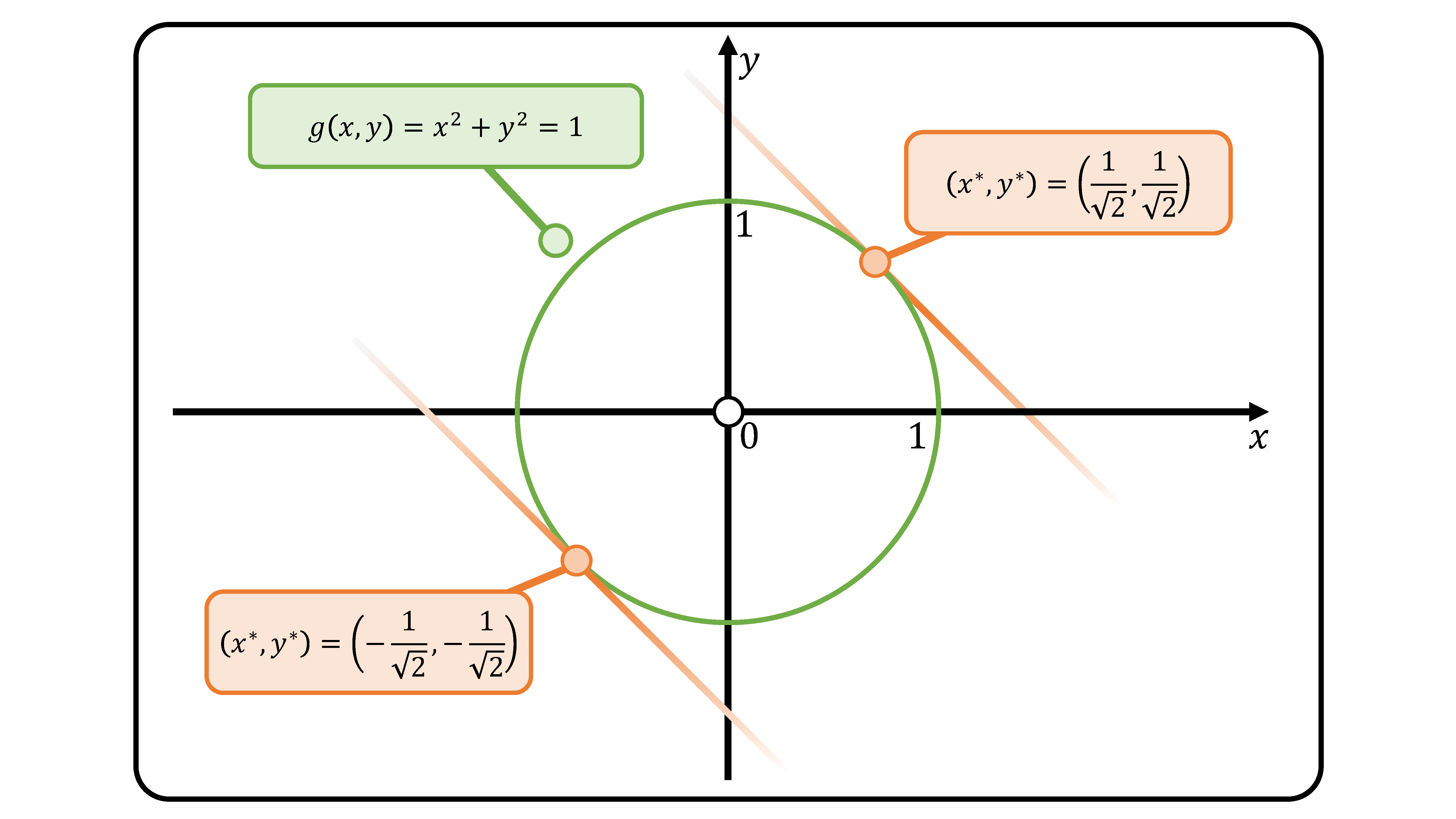
(Figure 1) Equality constraint \(g(x,y)=x^2+y^2=1\). The two optimal points for \(f(x,y)=x+y\).