Linear Systems — Introduction
Moses C. Nah
2023-03-04
Prelude
All models are wrong, but some are useful
In the field of science or engineering, it is a common practice to model the physical system or phenomenon in interest to a simpler, tractable and understandable mathematical formulation. One of the most basic and powerful formulations is to model the system in interest as a set of differential equations.
Depending on the system which we want to model, the set of differential equations could be either linear or nonlinear. A lumped-parameter model which consists of a mass-spring-damper can be described as a linear differential equation, while a frictionless pendulum under the influence of gravity cannot.
In this series of post, we specifically focus on linear systems, where the physical system in interest is described as the following set of linear differential equations.
\[ \begin{align*} \begin{split} \mathbf{\dot{x}}(t) &= \mathbf{A}(t)\mathbf{x}(t)+\mathbf{B}(t)\mathbf{u}(t)\\ \mathbf{y}(t) &= \mathbf{C}(t)\mathbf{x}(t)+\mathbf{D}(t)\mathbf{u}(t) \end{split} \tag{1} \end{align*} \] The notations of these equations are clarified in the this post.
One might be concerned that the baby is thrown with the bathwater, since linear differential equations seem too simple to contain the essential details of the system. Nevertheless, a lot of systems can be well-described by a collection of linear ordinary differential equations. Moreover, studying linear systems is a crucial stepping stone towards studying nonlinear systems. Hence, it is necessary to start with linear systems, which is the reason for this series of posts.
Analyzing the system in interest can be roughly divided into two steps (Figure 1):
- Modelling and obtaining the physical system as a set of linear differential equations
- Analyzing and studying those linear differential equations.
Here, we focus more on the second bullet, i.e., it is assumed that the mathematical model of the physical system in interest is given.
With the given linear mathematical model of the system, it is often necessary to control the behavior of the system in order to achieve a desired goal. This leads us to linear control theory, which is the main topic and protagonist of the posts. First and foremost, we introduce a rigorous derivation of the solution of \(\mathbf{x}(t)\) of Equation 1. For people who want to directly discuss about linear time-invariant systems, one can skip the previous post and start here..
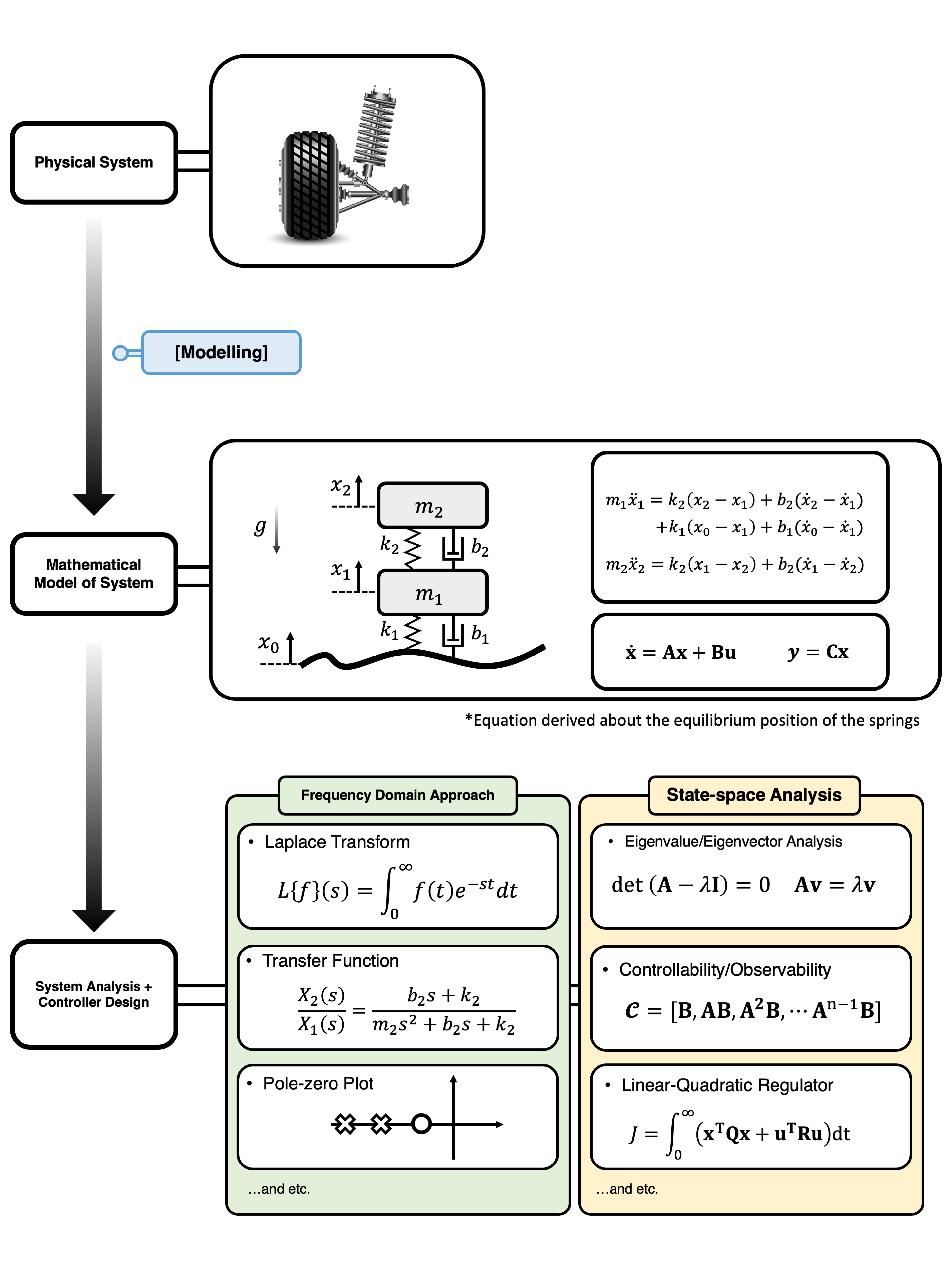
(Figure 1) The process of modelling and system analysis.
A Bit of History
There are two major divisions in control theory — Classical Control Theory and Modern Control Theory. Classical control theory uses frequency domain analysis by taking the Laplace transformation of the governing differential equations. On the other hand, modern control theory, which started at near late 1950s ~ early 1960s, uses the time-domain state-space representation (Equation 1), which is established by Rudolf Kalman [1] — the father of modern control theory. The seminal works from Kalman [2]–[5] have in fact, shifted the paradigm of control theory from the classical era to the modern era. In this series of post, we focus more on modern control theory, and we show the connection between these state-space methods and classical control theory. We are now ready to take a deep dive.
References
``